This is the final post in our three part series on shape detection and analysis.
Previously, we learned how to:
Today we are going to perform both shape detection and color labeling on objects in images.
At this point, we understand that regions of an image can be characterized by both color histograms and by basic color channel statistics such as mean and standard deviation.
But while we can compute these various statistics, they cannot give us an actual label such as “red”, “green”, “blue”, or “black” that tags a region as containing a specific color.
…or can they?
In this blog post, I’ll detail how we can leverage the L*a*b* color space along with the Euclidean distance to tag, label, and determine the color of objects in images using Python and OpenCV.
Looking for the source code to this post?
Jump right to the downloads section.
Determining object color with OpenCV
Before we dive into any code, let’s briefly review our project structure:
|--- pyimagesearch
|    |--- __init__.py
|    |--- colorlabeler.py
|    |--- shapedetector.py
|--- detect_color.py
|--- example_shapes.png
Notice how we are reusing the
shapedetector.pyand
ShapeDetectorclass from our previous blog post. We’ll also create a new file,
colorlabeler.py, that will be used to tag image regions with a text label of a color.
Finally, the
detect_color.pydriver script will be used to glue all the pieces together.
Before you continue working through this post, make sure that you have the imutils Python package installed on your system:
$ pip install imutils
We’ll be using various functions inside this library through the remainder of the lesson.
Labeling colors in images
The first step in this project is to create a Python class that can be used to label shapes in an image with their associated color.
To do this, let’s define a class named
ColorLabelerin the
colorlabeler.pyfile:
# import the necessary packages
from scipy.spatial import distance as dist
from collections import OrderedDict
import numpy as np
import cv2

class ColorLabeler:
	def __init__(self):
		# initialize the colors dictionary, containing the color
		# name as the key and the RGB tuple as the value
		colors = OrderedDict({
			"red": (255, 0, 0),
			"green": (0, 255, 0),
			"blue": (0, 0, 255)})

		# allocate memory for the L*a*b* image, then initialize
		# the color names list
		self.lab = np.zeros((len(colors), 1, 3), dtype="uint8")
		self.colorNames = []

		# loop over the colors dictionary
		for (i, (name, rgb)) in enumerate(colors.items()):
			# update the L*a*b* array and the color names list
			self.lab[i] = rgb
			self.colorNames.append(name)

		# convert the L*a*b* array from the RGB color space
		# to L*a*b*
		self.lab = cv2.cvtColor(self.lab, cv2.COLOR_RGB2LAB)
Line 2-5 imports our required Python packages while Line 7 defines the
ColorLabelerclass.
We then dive into the constructor on Line 8. To start, we need to initialize a colors dictionary (Lines 11-14) that specifies the mapping of the color name (the key to the dictionary) to the RGB tuple (the value of the dictionary).
From there, we allocate memory for a NumPy array to store these colors, followed by initializing the list of color names (Lines 18 and 19).
The next step is to loop over the
colorsdictionary, followed by updating the NumPy array and the
colorNameslist, respectively (Lines 22-25).
Finally, we convert the NumPy “image” from the RGB color space to the L*a*b* color space.
So why are we using the L*a*b* color space rather than RGB or HSV?
Well, in order to actually label and tag regions of an image as containing a certain color, we’ll be computing the Euclidean distance between our dataset of known colors (i.e., the
labarray) and the averages of a particular image region.
The known color that minimizes the Euclidean distance will be chosen as the color identification.
And unlike HSV and RGB color spaces, the Euclidean distance between L*a*b* colors has actual perceptual meaning — hence we’ll be using it in the remainder of this post.
The next step is to define the
labelmethod:
# import the necessary packages
from scipy.spatial import distance as dist
from collections import OrderedDict
import numpy as np
import cv2

class ColorLabeler:
	def __init__(self):
		# initialize the colors dictionary, containing the color
		# name as the key and the RGB tuple as the value
		colors = OrderedDict({
			"red": (255, 0, 0),
			"green": (0, 255, 0),
			"blue": (0, 0, 255)})

		# allocate memory for the L*a*b* image, then initialize
		# the color names list
		self.lab = np.zeros((len(colors), 1, 3), dtype="uint8")
		self.colorNames = []

		# loop over the colors dictionary
		for (i, (name, rgb)) in enumerate(colors.items()):
			# update the L*a*b* array and the color names list
			self.lab[i] = rgb
			self.colorNames.append(name)

		# convert the L*a*b* array from the RGB color space
		# to L*a*b*
		self.lab = cv2.cvtColor(self.lab, cv2.COLOR_RGB2LAB)

	def label(self, image, c):
		# construct a mask for the contour, then compute the
		# average L*a*b* value for the masked region
		mask = np.zeros(image.shape[:2], dtype="uint8")
		cv2.drawContours(mask, [c], -1, 255, -1)
		mask = cv2.erode(mask, None, iterations=2)
		mean = cv2.mean(image, mask=mask)[:3]

		# initialize the minimum distance found thus far
		minDist = (np.inf, None)

		# loop over the known L*a*b* color values
		for (i, row) in enumerate(self.lab):
			# compute the distance between the current L*a*b*
			# color value and the mean of the image
			d = dist.euclidean(row[0], mean)

			# if the distance is smaller than the current distance,
			# then update the bookkeeping variable
			if d < minDist[0]:
				minDist = (d, i)

		# return the name of the color with the smallest distance
		return self.colorNames[minDist[1]]
The
labelmethod requires two arguments: the L*a*b*
imagecontaining the shape we want to compute color channel statistics for, followed by
c, the contour region of the
imagewe are interested in.
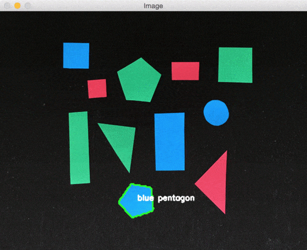
Lines 34 and 35 construct a mask for contour region, an example of which we can see below:
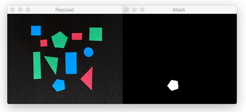
Figure 1: (Right) The original image. (Left) The mask image for the blue pentagon at the bottom of the image, indicating that we will only perform computations in the “white” region of the image, ignoring the black background.
Notice how the foreground region of the
maskis set to white, while the background is set to black. We’ll only perform computations within the masked (white) region of the image.
We also erode the mask slightly to ensure statistics are only being computed for the masked region and that no background is accidentally included (due to a non-perfect segmentation of the shape from the original image, for instance).
Line 37 computes the mean (i.e., average) for each of the L*, a*, and *b* channels of the
imagefor only the
mask‘ed region.
Finally, Lines 43-51 handles looping over each row of the
labarray, computing the Euclidean distance between each known color and the average color, and then returning the name of the color with the smallest Euclidean distance.
Defining the color labeling and shape detection process
Now that we have defined our
ColorLabeler, let’s create the
detect_color.pydriver script. Inside this script we’ll be combining both our
ShapeDetectorclass from last week and the
ColorLabelerfrom today’s post.
Let’s go ahead and get started:
# import the necessary packages
from pyimagesearch.shapedetector import ShapeDetector
from pyimagesearch.colorlabeler import ColorLabeler
import argparse
import imutils
import cv2

# construct the argument parse and parse the arguments
ap = argparse.ArgumentParser()
ap.add_argument("-i", "--image", required=True,
	help="path to the input image")
args = vars(ap.parse_args())
Lines 2-6 import our required Python packages — notice how we are importing both our
ShapeDetectorand
ColorLabeler.
Lines 9-12 then parse our command line arguments. Like the other two posts in this series, we only need a single argument: the
--imagepath where the image we want to process lives on disk.
Next up, we can load the image and process it:
# import the necessary packages
from pyimagesearch.shapedetector import ShapeDetector
from pyimagesearch.colorlabeler import ColorLabeler
import argparse
import imutils
import cv2

# construct the argument parse and parse the arguments
ap = argparse.ArgumentParser()
ap.add_argument("-i", "--image", required=True,
	help="path to the input image")
args = vars(ap.parse_args())

# load the image and resize it to a smaller factor so that
# the shapes can be approximated better
image = cv2.imread(args["image"])
resized = imutils.resize(image, width=300)
ratio = image.shape[0] / float(resized.shape[0])

# blur the resized image slightly, then convert it to both
# grayscale and the L*a*b* color spaces
blurred = cv2.GaussianBlur(resized, (5, 5), 0)
gray = cv2.cvtColor(blurred, cv2.COLOR_BGR2GRAY)
lab = cv2.cvtColor(blurred, cv2.COLOR_BGR2LAB)
thresh = cv2.threshold(gray, 60, 255, cv2.THRESH_BINARY)[1]

# find contours in the thresholded image
cnts = cv2.findContours(thresh.copy(), cv2.RETR_EXTERNAL,
	cv2.CHAIN_APPROX_SIMPLE)
cnts = cnts[0] if imutils.is_cv2() else cnts[1]

# initialize the shape detector and color labeler
sd = ShapeDetector()
cl = ColorLabeler()
Lines 16-18 handle loading the image from disk and then creating a
resizedversion of it, keeping track of the
ratioof the original height to the resized height. We resize the image so that our contour approximation is more accurate for shape identification. Furthermore, the smaller the image is, the less data there is to process, thus our code will execute faster.
Lines 22-25 apply Gaussian smoothing to our resized image, converting to grayscale and L*a*b*, and finally thresholding to reveal the shapes in the image:
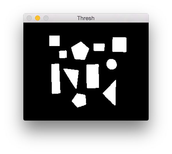
Figure 2: Thresholding is applied to segment the background from the foreground shapes.
We find the contours (i.e., outlines) of the shapes on Lines 29-30, taking care of to grab the appropriate tuple value of
cntsbased on our OpenCV version.
We are now ready to detect both the shape and color of each object in the image:
# import the necessary packages
from pyimagesearch.shapedetector import ShapeDetector
from pyimagesearch.colorlabeler import ColorLabeler
import argparse
import imutils
import cv2

# construct the argument parse and parse the arguments
ap = argparse.ArgumentParser()
ap.add_argument("-i", "--image", required=True,
	help="path to the input image")
args = vars(ap.parse_args())

# load the image and resize it to a smaller factor so that
# the shapes can be approximated better
image = cv2.imread(args["image"])
resized = imutils.resize(image, width=300)
ratio = image.shape[0] / float(resized.shape[0])

# blur the resized image slightly, then convert it to both
# grayscale and the L*a*b* color spaces
blurred = cv2.GaussianBlur(resized, (5, 5), 0)
gray = cv2.cvtColor(blurred, cv2.COLOR_BGR2GRAY)
lab = cv2.cvtColor(blurred, cv2.COLOR_BGR2LAB)
thresh = cv2.threshold(gray, 60, 255, cv2.THRESH_BINARY)[1]

# find contours in the thresholded image
cnts = cv2.findContours(thresh.copy(), cv2.RETR_EXTERNAL,
	cv2.CHAIN_APPROX_SIMPLE)
cnts = cnts[0] if imutils.is_cv2() else cnts[1]

# initialize the shape detector and color labeler
sd = ShapeDetector()
cl = ColorLabeler()

# loop over the contours
for c in cnts:
	# compute the center of the contour
	M = cv2.moments(c)
	cX = int((M["m10"] / M["m00"]) * ratio)
	cY = int((M["m01"] / M["m00"]) * ratio)

	# detect the shape of the contour and label the color
	shape = sd.detect(c)
	color = cl.label(lab, c)

	# multiply the contour (x, y)-coordinates by the resize ratio,
	# then draw the contours and the name of the shape and labeled
	# color on the image
	c *= ratio
	text = "{} {}".format(color, shape)
	cv2.drawContours(image, [c], -1, (0, 255, 0), 2)
	cv2.putText(image, text, (cX, cY),
		cv2.FONT_HERSHEY_SIMPLEX, 0.5, (255, 255, 255), 2)

	# show the output image
	cv2.imshow("Image", image)
	cv2.waitKey(0)
We start looping over each of the contours on Line 37, while Lines 39-41 compute the center of the shape.
Using the contour, we can then detect the
shapeof the object, followed by determining its
coloron Lines 44-45.
Finally, Lines 50-54 handle drawing the outline of the current shape, followed by the color + text label on the output image.
Lines 57 and 58 display the results to our screen.
Color labeling results
To run our shape detector + color labeler, just download the source code to the post using the form at the bottom of this tutorial and execute the following command:
$ python detect_color.py --image example_shapes.png
Figure 3: Detecting the shape and labeling the color of objects in an image.
As you can see from the GIF above, each object has been correctly identified both in terms of shape and in terms of color.
Limitations
One of the primary drawbacks to using the method presented in this post to label colors is that due to lighting conditions, along with various hues and saturations, colors rarely look like pure red, green, blue, etc.
You can often identify small sets of colors using the L*a*b* color space and the Euclidean distance, but for larger color palettes, this method will likely return incorrect results depending on the complexity of your images.
So, that being said, how can we more reliably label colors in images?
Perhaps there is a way to “learn” what colors “look like” in the real-world.
Indeed, there is.
And that’s exactly what I’ll be discussing in a future blog post.
Summary
Today is the final post in our three part series on shape detection and analysis.
We started by learning how to compute the center of a contour using OpenCV. Last week we learned how to utilize contour approximation to detect shapes in images. And finally, today we combined our shape detection algorithm with a color labeler, used to tag shapes a specific color name.
While this method works for small color sets in semi-controlled lighting conditions, it will likely not work for larger color palettes in less controlled environments. As I hinted at in the “Limitations” section of this post, there is actually a way for us to “learn” what colors “look like” in the real-world. I’ll save the discussion of this method for a future blog post.
So, what did you think of this series of blog posts? Be sure to let me know in the comments section.
And be sure to signup for the PyImageSearch Newsletter using the form below to be notified when new posts go live!
Downloads:
The post Determining object color with OpenCV appeared first on PyImageSearch.