Quantcast
Channel: OpenCV 3 – PyImageSearch
Viewing all 49 articles
Browse latest View live

OpenCV 3.0 released — and the coming changes to the PyImageSearch blog.

$
0
0

opencv3_installed_examples

It’s been a long time coming, but OpenCV 3.0 has finally been released!

This update is definitely one of the most extensive overhauls to the library in recent years, and boasts increased stability, performance increases, and OpenCL support.

But by far, the most exciting update for us in the Python world is:

Python 3 support!

After years of being stuck in Python 2.7, we can now finally use OpenCV in Python 3.0! Awesome news indeed!

So you might be asking “What does this mean for PyImageSearch?”

Are we dropping OpenCV 2.4.X immediately and moving to OpenCV 3.0? Are we officially done with Python 2.7?

The short answer is no.

OpenCV 3.0 being released is awesome news — but this is also a transition time for the computer vision community. Some of us will be dependent on the previous OpenCV 2.4.X version. Others will be dashing to grab the latest bleeding-edge copy of v3.0. And perhaps others of us won’t really care what version we are using provided that our code executes and runs as expected.

Because of these variety of reasons, moving forward I will be writing content related to both OpenCV 2.4.X and OpenCV 3.0.

I think it would be a huge mistake to abandon writing content on OpenCV 2.4.X right now. It’s older. It’s more established. And it’s more widely used.

However, it would be an equally huge mistake to ignore OpenCV 3.0 until it matures and gets a few minor releases under its belt. OpenCV 3.0 is indeed the future — and we need to treat it as such.

Because of this, I have come up with the following plan:

We’ll be doing a mix of OpenCV 2.4.X and OpenCV 3.0.

OpenCV 3.0 is brand new. It’s shiny. It’s sexy. We’ll definitely be taking off the wrapper and having some fun.

But we’ll still be doing a fair amount of tutorials in OpenCV 2.4.X. Remember, OpenCV 2.4.X is still the de facto library for computer vision and image processing and will remain so until the v3.0 matures a little bit and obtains a substantial adoption rate.

All new blog posts will be marked with OpenCV + Python versions.

All new articles, tutorials, and blog posts published on PyImageSearch will include both the assumed OpenCV version and Python version to ensure that you know which development environment we are using.

You can also expect some OpenCV 3.0 install tutorials on a variety of platforms coming soon.

All old blog posts will also be marked with OpenCV + Python versions.

Just like all new posts will list the assumed versions of OpenCV and Python, I will also be going back and updating all old blog posts to include the required versions of OpenCV and Python.

This change will not happen overnight, but I’ll be updating a few older articles per week.

The updated posts will include a section like this:

Figure 1: All blog posts on PyImageSearch will include a section that explicitly defines which Python and OpenCV versions are being used.

Figure 1: All blog posts on PyImageSearch will include a section that explicitly defines which Python and OpenCV versions are being used.

What about Practical Python and OpenCV + Case Studies?

You might be wondering about my books, Practical Python and OpenCV + Case Studies — will they be updated to OpenCV 3.0?

The answer is YES, Practical Python and OpenCV + Case Studies will absolutely be updated to cover OpenCV 3.0.

I have already forked the example code from the books and am updating the code examples.

The first update to the book will include revised source code for those who want to run the provided examples using Python 3 and OpenCV 3.0.

The second update will then transition the actual code explanations in the book to OpenCV 3.0.

I will likely be providing both a 2.4.X and 3.0 version of the book.

Regardless, the update OpenCV will in no way harm the integrity of Practical Python and OpenCV + Case Studies. Definitely consider purchasing a copy if you want to get up to speed on OpenCV. As I promised above, the book will be updated to cover OpenCV 3.0 as well.

There will be a transition period.

As I mentioned in the sections above, we will be doing a mix of OpenCV 2.4.X and OpenCV 3.0 articles and tutorials.

In the beginning most of these tutorials will be using the 2.4.X version.

But as the OpenCV 3.0 matures, we’ll mature with it and start introducing more and more v3.0 tutorials.

Exactly how long will the transition period take?

It’s hard to put an exact timeline on the transition period since it depends on a variety of factors:

  • It depends on how willing developers and programmers are to update to a new version of OpenCV and risk legacy code breaking (which based on my initial tests, that risk is very high).

  • It depends on the actual demand of OpenCV 3.0 tutorials.

  • And it depends on your feedback

My guess is that it could take up to 6-12 months before we use OpenCV 3.0 regularly on PyImageSearch, but who knows — my estimate could be way off. It could be shorter. And it could be longer.

Realistically, my gut tells me that we won’t be fully transitioning over until the 3.1 release. Remember, PyImageSearch is a teaching blog, and thus it’s very important that all of the code examples work as advertised.

Either way, my promise to you is that I’ll evolve the PyImageSearch blog as OpenCV evolves — and we’ll continue to ensure that PyImageSearch is the go to website to learn computer vision + OpenCV.

If anything, the only real change you’ll see is more posts from me.

I think the only big change you’ll see on the PyImageSearch blog is perhaps more blog posts.

Each Monday I’ll continue publishing the big blog post for the week. And then you might see another short blog post later in the week that details a particular caveat of OpenCV 3.0. As I said, this will be a transition period and each post published will detail the assumed Python and OpenCV versions.

So what do you think?

Do you like the plan? Hate the plan?

Leave a comment or shoot me a message — your input and response is what makes this blog possible!

The post OpenCV 3.0 released — and the coming changes to the PyImageSearch blog. appeared first on PyImageSearch.


Install OpenCV 3.0 and Python 2.7+ on OSX

$
0
0

face_detection_opencv3

As I mentioned last week, OpenCV 3.0 is finally here!

And if you’ve been paying attention to my Twitter stream, you may have noticed a bunch of tweets regarding installing OpenCV on OSX and Ubuntu (yep, I’ve been tweeting a lot lately, but that’s just because I’m so excited about the 3.0 release!)

To celebrate OpenCV 3.0, I have decided to perform a series of blog posts that detail how to install OpenCV 3.0 on both Python 2.7+ and Python 3+.

We’ll also be performing these Python 2.7 and Python 3+ installations on a variety of platforms including OSXUbuntu, and yes, the Raspberry Pi.

As I’m sure you already know, OpenCV has never been an effortless library to install. It’s not like you can let

pip
  or
easy_install
  to the heavy-lifting for you. In most cases you’ll be pulling down the repo, installing prerequisites, compiling by hand, and hoping that your installation goes smoothly.

With OpenCV 3.0 it doesn’t get any easier — and there are definitely some caveats and gotchas that you need to look out for (such as the opencv_contrib repository — without it, you’ll be missing out on some important features, such as SIFT, SURF, etc.)

But don’t worry, I’ve got you covered! Just keep following along with the PyImageSearch blog and I promise these tutorials will get you up and running with OpenCV 3.0 in no time.

We’ll go ahead and kick-off our OpenCV 3.0 install fest by installing v3.0 with Python 2.7+ bindings on the OSX platform.

If you’re an Ubuntu or Raspberry Pi user, be sure to keep an eye on PyImageSearch as I’ll be posting OpenCV 3.0 install instructions for Ubuntu and the Raspberry Pi as well.

A quick note before we get started: While OpenCV 3.0 is indeed compatible with Python 3+, most computer vision developers are still using Python 2.7 (since OpenCV 2.4.X is only compatible with Python 2.7). If you’re a Python 3 user and excited to give the bindings a try — don’t worry! I’ll be covering OpenCV 3.0 and Python 3+ installation in a future tutorial. But for now, let’s stick with what we know and use Python 2.7.

How to Install OpenCV 3.0 and Python 2.7+ on OSX

This is our first tutorial in our OpenCV 3.0 install-fest series. In this tutorial I’ll be detailing how to install OpenCV 3.0 and Python 2.7+ on the OSX operating system — I’ll be covering Python 3+ in a future post.

Let’s go ahead and dive into the OpenCV 3.0 and Python 2.7+ install instructions.

Step 1:

The first step we need to do is install Xcode, which is a combination of IDE and software development tools for developing applications on the OSX and iOS platforms — most of us already have Xcode installed.

But if you don’t, you’ll want to open up the App Store application and search for Xcode. From there, just click Get and Install App (and when prompted, you’ll need to enter your Apple ID username and password):

Figure 1: Installing Xcode on your OSX system.

Figure 1: Installing Xcode on your OSX system.

Step 2:

Now that Xcode is installed, we need to install Homebrew, which is labeled as “The missing package manager for OSX” (and they really are not joking about that one). Think of Homebrew as an (almost) equivalent of apt-get for Ubuntu.

To install Homebrew, simply head to the Homebrew website and simply copy and paste the command underneath the “Install Homebrew” section into your terminal:

$ cd ~
$ $ ruby -e "$(curl -fsSL https://raw.githubusercontent.com/Homebrew/install/master/install)"

Now that Homebrew is installed, you’ll need to update it and grab the latest package (i.e. “formula”) definitions. These formula are simply instructions on how to install a given package or library.

To update Homebrew, simply execute:

$ brew update

Step 3:

It’s bad form to use the system Python as your main interpreter. And this is especially true if you intend on using

virtualenv
  and
virtualenvwrapper
  (which we will be).

Let’s go ahead and use Homebrew to install our user-specific version of Python 2.7:

$ brew install python

Note: This tutorial will be covering how to install and setup OpenCV 3.0 with Python 2.7. I will be covering how to install OpenCV 3.0 with Python 3+ later this month.

However, before we proceed, we need to update our

PATH
  in our
~/.bash_profile
  file to indicate that we want to use Homebrew packages before any system libraries or packages. This is an absolutely critical step, so be sure not to skip it!

Open up your

~/.bash_profile
  file in your favorite editor (if it does not exist, create it), and append the following lines to the file:
# Homebrew
export PATH=/usr/local/bin:$PATH

From there, reload your

~./bash_profile
  file to ensure the changes have been made:
$ source ~/.bash_profile

As a sanity check, let’s confirm that we are using the Homebrew version of Python rather than the system one:

$ which python
/usr/local/bin/python

If your output of

which python
  is
/usr/local/bin/python
 , then you are indeed using the Homebrew version of Python. And if your output is
/usr/bin/python
 , then you are still using the system version of Python — and you need to go back and ensure that your
~/.bash_profile
  file is updated and reloaded correctly.

Again, this is a very important step, so be sure not to skip it!

Step 4:

Alright, time to get virtualenv and virtualenvwrapper installed and configured correctly. These packages allow us to create separate Python environments for each project we are working on. This is especially useful if you have projects that require different (or conflicting) versions of a given library.

It’s important to note that

virtualenv
  and
virtualenvwrapper
  are by no means required to install OpenCV 3.0 and Python 2.7+ on OSX. However, you really should be using these packages when doing Python development. It’s cleaner. Easier to maintain. And well worth the upfront effort.

Anyway, to install

virtualenv
  and
virtualenvwrapper
 , just execute the following command:
$ pip install virtualenv virtualenvwrapper

Again, we need to update our

~/.bash_profile
  file by appending the following two lines:
# Virtualenv/VirtualenvWrapper
source /usr/local/bin/virtualenvwrapper.sh

After updating the

~/.bash_profile
  file, we need to reload it:
$ source ~/.bash_profile

At this point, both

virtualenv
  and
virtualenvwrapper
  are installed correctly, so we can create our
cv
  virtual environment:
$ mkvirtualenv cv

This command will create a new Python environment that is entirely sequestered from our system and Homebrew Python installations. The

cv
  virtual environment is where we’ll be doing all of our computer vision development (and not to mention, compiling OpenCV 3.0 with Python 2.7+ support).

Step 5:

Now we can start installing some Python packages. We need to install NumPy since the OpenCV Python bindings represent images as multi-dimensional NumPy arrays:

$ pip install numpy

Step 6:

Up until this point we have been mainly focusing on actually setting up and configuring our development environment to compile and install OpenCV — here is where the real work starts.

First, we’ll use brew to install the required developers tools, such as the wonderful CMake utility:

$ brew install cmake pkg-config

And here we are going to install the necessary image I/O packages. These packages allow you to load various image file formats such as JPEG, PNG, TIFF, etc.

$ brew install jpeg libpng libtiff openexr

And finally, let’s install libraries that are used to optimize various operations within OpenCV (if we so choose):

$ brew install eigen tbb

Step 7:

Alright, our system is all setup — time to compile and install OpenCV 3.0 with Python 2.7+ support.

The first thing we’ll do is change directory to our home directory, followed by pulling down OpenCV from GitHub, and checking out the

3.0.0
  version:
$ cd ~
$ git clone https://github.com/Itseez/opencv.git
$ cd opencv
$ git checkout 3.0.0

Unlike previous versions of OpenCV that were (essentially) self-contained, we need to pull down the extra opencv_contrib repo from GitHub as well. The

opencv_contrib
  repo which contains extra modules for OpenCV, such as feature detection, local invariant descriptors (SIFT, SURF, etc.), text detection in natural images, line descriptors, and more.
$ cd ~
$ git clone https://github.com/Itseez/opencv_contrib
$ cd opencv_contrib
$ git checkout 3.0.0

Note: We don’t have to pull down the

opencv_contrib
  repo if we don’t want to. OpenCV will compile and install just fine without it. But if you compile OpenCV without
opencv_contrib
 , be warned that you’ll be missing out on some pretty important features, which will become very obvious, very fast, especially if you’re used to working with the 2.4.X version of OpenCV.

Step 8:

Let’s setup our OpenCV build by creating the

build
  directory:
$ cd ~/opencv
$ mkdir build
$ cd build

Where we’ll use CMake to configure our build:

$ cmake -D CMAKE_BUILD_TYPE=RELEASE -D CMAKE_INSTALL_PREFIX=/usr/local \
	-D PYTHON2_PACKAGES_PATH=~/.virtualenvs/cv/lib/python2.7/site-packages \
	-D PYTHON2_LIBRARY=/usr/local/Cellar/python/2.7.10/Frameworks/Python.framework/Versions/2.7/bin \
	-D PYTHON2_INCLUDE_DIR=/usr/local/Frameworks/Python.framework/Headers \
	-D INSTALL_C_EXAMPLES=ON -D INSTALL_PYTHON_EXAMPLES=ON \
	-D BUILD_EXAMPLES=ON \
	-D OPENCV_EXTRA_MODULES_PATH=~/opencv_contrib/modules ..

There are some very important options we are supplying to CMake here, so let’s break them down:

  • CMAKE_BUILD_TYPE
     : This option indicates that we are building a release binary of OpenCV.
  • CMAKE_INSTALL_PREFIX
     : The base directory where OpenCV will be installed.
  • PYTHON2_PACKAGES_PATH
     : The explicit path to where our
    site-packages
      directory lives in our
    cv
      virtual environment.
  • PYTHON2_LIBRARY
     : Path to our Hombrew installation of Python.
  • PYTHON2_INCLUDE_DIR
     : The path to our Python header files for compilation.
  • INSTALL_C_EXAMPLES
     : Indicate that we want to install the C/C++ examples after compilation.
  • INSTALL_PYTHON_EXAMPLES
     : Indicate that we want to install the Python examples after complication.
  • BUILD_EXAMPLES
     : A flag that determines whether or not the included OpenCV examples will be compiled or not.
  • OPENCV_EXTRA_MODULES_PATH
     : This option is extremely important — here we supply the path to the
    opencv_contrib
      repo that we pulled down earlier, indicating that OpenCV should compile the extra modules as well.

Whew, that was a lot of options.

Trust me, it’s a lot easier installing OpenCV 3.0 on Ubuntu where these options are automatically determined via CMake for us.

But when using OSX you’ll need to explicitly define the

PYTHON2_PACKAGES_PATH
 ,
PYTHON2_LIBRARY
 , and
PYTHON2_INCLUDE_DIR
  yourself. It’s a real pain, but if you don’t, your compile will fail.

Here’s an example of what my CMake output looks like:

Figure 2: Before compiling OpenCV 3.0 on your OSX system, make sure that cmake has picked up the correct Python interpreter, library, numpy version, and packages path.

Figure 2: Before compiling OpenCV 3.0 on your OSX system, make sure that cmake has picked up the correct Python interpreter, library, numpy version, and packages path.

Notice how the Python 2 Interpreter, Libraries, numpy version, and packages path have been correctly picked up.

You’ll also want to make sure that

python2
  is in the list of modules To be built, like this:
Figure 2: Ensuring the "python2" module is in our list of modules "To be built".

Figure 2: Ensuring the “python2” module is in our list of modules “To be built”.

If it

python2
  is not in this list, and is in the Unavailable list, then you need to go back to the CMake step and ensure that you have correctly supplied your
PYTHON2_PACKAGES_PATH
 ,
PYTHON2_LIBRARY
 , and
PYTHON2_INCLUDE_DIR
 .

Now that CMake has properly configured the build, we can compile OpenCV:

$ make -j4

Where the 4 can be replaced with however many cores you have available on your processor. Here’s an example of OpenCV compiling on my system:

Figure 3: OpenCV 3.0 with Python 2.7+ support compiling on my system.

Figure 3: OpenCV 3.0 with Python 2.7+ support compiling on my system.

And assuming that OpenCV compiled without error, you can now install it on your OSX system:

$ make install

If you get an error message related to permissions (although that really shouldn’t happen), you’ll need to run the install command as

sudo
 :
$ sudo make install

Step 9:

Assuming you’ve made it this far, let’s perform a sanity check and ensure OpenCV is installed:

$ cd ~/.virtualenvs/cv/lib/python2.7/site-packages/
$ ls -l cv2.so 
-rwxr-xr-x  1 adrian  staff  2013052 Jun  5 15:20 cv2.so

Sure enough, we can see that OpenCV has been installed in our

cv
  virtual environment’s
site-packages
  directory!

As a quick note, you’ll be able to find the

cv2.so
  file (which is your OpenCV bindings) in your
build/lib
  directory as well.

Let’s verify our install by firing up a shell and importing OpenCV:

(cv)annalee:~ adrianrosebrock$ python
Python 2.7.8 (default, Jul 31 2014, 15:41:09) 
[GCC 4.2.1 Compatible Apple LLVM 5.1 (clang-503.0.40)] on darwin
Type "help", "copyright", "credits" or "license" for more information.
>>> import cv2
>>> cv2.__version__
'3.0.0'

Doesn’t that

3.0.0
  look nice?

Congrats, you have now installed OpenCV 3.0 and Python 2.7+ on your OSX system!

Step 10:

After all this work, let’s give our OpenCV 3.0 install a test drive!

Most of my work in computer vision involves image search engines, or more formally, Content-based Image Retrieval. A critical step of CBIR is extracting features to quantify and abstractly represent the contents of an image.

OpenCV 3.0 has numerous updates and changes, but perhaps my personal favorite is an implementation of AKAZE features — Fast Explicit Diffusion for Accelerated Features in Nonlinear Scale Spaces by Alcantarilla et al.

Since Jurassic World was just released (and Jurassic Park is my favorite movie of all time), let’s explore how we can compute and extract AKAZE features from the following image:

Figure 4: Our Jurassic World test image that we are going to detect keypoints and extract features using AKAZE.

Figure 4: Our Jurassic World test image that we are going to detect keypoints and extract features in using AKAZE.

Open up a new file, name it

test_akaze.py
 , and insert the following code:
# import the necessary packages
from __future__ import print_function
import cv2

# load the image and convert it to grayscale
image = cv2.imread("jurassic_world.jpg")
gray = cv2.cvtColor(image, cv2.COLOR_BGR2GRAY)
cv2.imshow("Original", image)

# initialize the AKAZE descriptor, then detect keypoints and extract
# local invariant descriptors from the image
detector = cv2.AKAZE_create()
(kps, descs) = detector.detectAndCompute(gray, None)
print("keypoints: {}, descriptors: {}".format(len(kps), descs.shape))

# draw the keypoints and show the output image
cv2.drawKeypoints(image, kps, image, (0, 255, 0))
cv2.imshow("Output", image)
cv2.waitKey(0)

And then execute it via:

$ python test_akaze.py
keypoints: 762, descriptors: (762, 61)

Assuming you have download the

jurassic_world.jpg
  image and placed it in the same directory as your
test_akaze.py
  script, you should see the following output:
Figure 5: We have successfully been able to detect keypoints, extract AKAZE features, and then draw the keypoints on our image using OpenCV 3.0 and Python 2.7+!

Figure 5: We have successfully been able to detect keypoints, extract AKAZE features, and then draw the keypoints on our image using OpenCV 3.0 and Python 2.7+!

Notice how we have been able to detect keypoints and extract AKAZE features in our image!

Obviously we need to do a lot more work than this to build a useful project using AKAZE features — but this example demonstrates that (1) our OpenCV 3.0 install is working, and (2) we are able to use a unique OpenCV 3.0 feature using Python 2.7.

Summary

OpenCV 3.0 is finally here! And to celebrate the OpenCV 3.0 release, we are going to performing an OpenCV 3.0 install-fest for both Python 2.7+ and Python 3+ on a variety of operating systems including OSXUbuntu, and the Raspberry Pi!

This article kicked-off the install fest by detailing how to setup and install OpenCV 3.0 and Python 2.7+ on the OSX operating system.

Next week, we’ll be moving over to Ubuntu and detailing the instructions to get OpenCV 3.0 and Python 2.7 installed on Ubuntu 14.04+ (hint: it’s much easier than OSX).

Anyway, I hope you enjoyed this post and found it useful!

Please consider subscribing to the PyImageSearch Newsletter by entering your email address in the form below — I’ll be sending out updates as new OpenCV 3.0 + Python install instructions are released!

The post Install OpenCV 3.0 and Python 2.7+ on OSX appeared first on PyImageSearch.

Install OpenCV 3.0 and Python 2.7+ on Ubuntu

$
0
0

opencv3_handwriting_reco

Last week we kicked-off the OpenCV 3.0 install fest by detailing how to install OpenCV 3.0 and Python 2.7+ on the OSX platform.

Today we are going to continue the OpenCV 3.0 install instruction series by moving over to the Ubuntu operating system.

In the remainder of the post I will provide instructions on how to configure and install OpenCV 3.0 and Python 2.7+ on Ubuntu. I have personally tested these instructions on Ubuntu 14.04, but they should pretty much work on any Debian-based operating system.

A quick note before we get started: Yes, OpenCV 3.0 is indeed compatible with Python 3+. However, the install instructions are slightly different between Python 2.7+ and Python 3+. In an effort to keep each article self-contained and easy to follow, I am creating separate OpenCV 3.0 install tutorials for Python 2.7 and Python 3+. If you would like to use OpenCV 3.0 and Python 3+ on your Ubuntu system, please keep an eye on this blog — I will be posting OpenCV 3.0 and Python 3+ install instructions later this month. But for the time being, let’s stick with Python 2.7.

How to Install OpenCV 3.0 and Python 2.7+ on Ubuntu

This is the second article in the OpenCV 3.0 install-fest series. Last week we covered how to install OpenCV 3.0 and Python 2.7+ on OSX. Today we are going to perform the same OpenCV 3.0 and Python 2.7 installation, only on the Ubuntu operating system. In general, you should find installing OpenCV 3.0 and Python 2.7+ on Ubuntu much easier than installing on OSX.

Step 1:

Open up a terminal and update the

apt-get
  package manager followed by upgrading any pre-installed packages:
$ sudo apt-get update
$ sudo apt-get upgrade

Step 2:

Now we need to install our developer tools:

$ sudo apt-get install build-essential cmake git pkg-config

The

pkg-config
  is likely already installed, but be sure to include it just in case. We’ll be using
git
  to pull down the OpenCV repositories from GitHub. The 
cmake
  package is used to configure our build.

Step 3:

OpenCV needs to be able to load various image file formats from disk, including JPEG, PNG, TIFF, etc. In order to load these image formats from disk, we’ll need our image I/O packages:

$ sudo apt-get install libjpeg8-dev libtiff4-dev libjasper-dev libpng12-dev

Step 4:

At this point, we have the ability to load a given image off of disk. But how do we display the actual image to our screen? The answer is the GTK development library, which the

highgui
  module of OpenCV depends on to guild Graphical User Interfaces (GUIs):
$ sudo apt-get install libgtk2.0-dev

Step 5:

We can load images using OpenCV, but what about processing video streams and accessing individual frames? We’ve got that covered here:

$ sudo apt-get install libavcodec-dev libavformat-dev libswscale-dev libv4l-dev

Step 6:

Install libraries that are used to optimize various routines inside of OpenCV:

$ sudo apt-get install libatlas-base-dev gfortran

Step 7:

Install

pip
 , a Python package manager:
$ wget https://bootstrap.pypa.io/get-pip.py
$ sudo python get-pip.py

Step 8:

Install virtualenv and virtualenvwrapper. These two packages allow us to create separate Python environments for each project we are working on. While installing

virtualenv
  and
virtualenvwrapper
  is not a requirement to get OpenCV 3.0 and Python 2.7+ up and running on your Ubuntu system, I highly recommend it and the rest of this tutorial will assume you have them installed!
$ sudo pip install virtualenv virtualenvwrapper
$ sudo rm -rf ~/.cache/pip

Now that we have

virtualenv
  and
virtualenvwrapper
  installed, we need to update our
~/.bashrc
  file:
# virtualenv and virtualenvwrapper
export WORKON_HOME=$HOME/.virtualenvs
source /usr/local/bin/virtualenvwrapper.sh

This quick update will ensure that both

virtualenv
  and
virtualenvwrapper
  are loaded each time you login.

To make the changes to our

~/bashrc
  file take affect, you can either (1) logout and log back in, (2) close your current terminal window and open a new one, or preferably, (3) reload the contents of your
~/.bashrc
  file:
$ source ~/.bashrc

Lastly, we can create our

cv
  virtual environment where we’ll be doing our computer vision development and OpenCV 3.0 + Python 2.7+ installation:
$ mkvirtualenv cv

Step 9:

As I mentioned above, this tutorial covers how to install OpenCV 3.0 and Python 2.7+ (I’ll have a OpenCV 3.0 + Python 3 tutorial available later this month), so we’ll need to install our Python 2.7 development tools:

$ sudo apt-get install python2.7-dev

Since OpenCV represents images as multi-dimensional NumPy arrays, we better install NumPy into our

cv
  virtual environment:
$ pip install numpy

Step 10:

Our environment is now all setup — we can proceed to change to our home directory, pull down OpenCV from GitHub, and checkout the

3.0.0
  version:
$ cd ~
$ git clone https://github.com/Itseez/opencv.git
$ cd opencv
$ git checkout 3.0.0

As I mentioned last week, we also need the opencv_contrib repo as well. Without this repository, we won’t have access to standard keypoint detectors and local invariant descriptors (such as SIFT, SURF, etc.) that were available in the OpenCV 2.4.X version. We’ll also be missing out on some of the newer OpenCV 3.0 features like text detection in natural images:

$ cd ~
$ git clone https://github.com/Itseez/opencv_contrib.git
$ cd opencv_contrib
$ git checkout 3.0.0

Time to setup the build:

$ cd ~/opencv
$ mkdir build
$ cd build
$ cmake -D CMAKE_BUILD_TYPE=RELEASE \
	-D CMAKE_INSTALL_PREFIX=/usr/local \
	-D INSTALL_C_EXAMPLES=ON \
	-D INSTALL_PYTHON_EXAMPLES=ON \
	-D OPENCV_EXTRA_MODULES_PATH=~/opencv_contrib/modules \
	-D BUILD_EXAMPLES=ON ..

Notice how compared to last week our CMake command is substantially less verbose and requires less manual tweaking — this is because CMake is able to better automatically tune our install parameters (at least compared to OSX).

Now we can finally compile OpenCV:

$ make -j4

Where you can replace the 4 with the number of available cores on your processor to speedup the compilation.

Here’s an example of OpenCV 3.0 compiling on my system:

Figure 1: OpenCV 3.0 with Python 2.7+ support compiling on my Ubuntu 14.04 system.

Figure 1: OpenCV 3.0 with Python 2.7+ support compiling on my Ubuntu 14.04 system.

Assuming that OpenCV compiled without error, you can now install it on your Ubuntu system:

$ sudo make install
$ sudo ldconfig

Step 11:

If you’ve reached this step without an error, OpenCV should now be installed in 

/usr/local/lib/python2.7/site-packages

However, our

cv
  virtual environment is located in our home directory — thus to use OpenCV within our
cv
  environment, we first need to sym-link OpenCV into the
site-packages
  directory of the
cv
  virtual environment:
$ cd ~/.virtualenvs/cv/lib/python2.7/site-packages/
$ ln -s /usr/local/lib/python2.7/site-packages/cv2.so cv2.so

Step 12:

Congratulations! You have successfully installed OpenCV 3.0 with Python 2.7+ bindings on your Ubuntu system!

To confirm your installation, simply ensure that you are in the

cv
  virtual environment, followed by importing
cv2
 :
$ workon cv
$ python
>>> import cv2
>>> cv2.__version__
'3.0.0'

Here’s an example of demonstrating the OpenCV 3.0 and Python 2.7+ install on my own Ubuntu machine:

Figure 2: OpenCV 3.0 with Python 2.7+ bindings has been successfully installed on Ubuntu!

Figure 2: OpenCV 3.0 with Python 2.7+ bindings has been successfully installed on Ubuntu!

Step 13:

Now that OpenCV has been configured and installed, let’s build a quick Python script to detect the red game cartridge in the image named

games.jpg
  below:
Figure 2: Our goal is to detect the red game cartridge (on the right) in this image.

Figure 3: Our goal is to detect the red game cartridge (on the right) in this image.

Open up your favorite editor, create a new file, name it

find_game.py
 , and insert the following code:
# import the necessary packages
import numpy as np
import cv2

# load the games image
image = cv2.imread("games.jpg")

# find the red color game in the image
upper = np.array([65, 65, 255])
lower = np.array([0, 0, 200])
mask = cv2.inRange(image, lower, upper)

# find contours in the masked image and keep the largest one
(_, cnts, _) = cv2.findContours(mask.copy(), cv2.RETR_EXTERNAL,
	cv2.CHAIN_APPROX_SIMPLE)
c = max(cnts, key=cv2.contourArea)

# approximate the contour
peri = cv2.arcLength(c, True)
approx = cv2.approxPolyDP(c, 0.05 * peri, True)

# draw a green bounding box surrounding the red game
cv2.drawContours(image, [approx], -1, (0, 255, 0), 4)
cv2.imshow("Image", image)
cv2.waitKey(0)

You’ll also need to download the games.jpg image and place it in the same directory as your

find_game.py
  file. Once the
games.jpg
  file has been downloaded, you can execute the script via:
$ python find_game.py

Assuming that you have downloaded the

games.jpg
  image and placed it in the same directory as our
find_game.py
  script, you should see the following output:
Figure 4: We have successfully detected the red game cartridge in the image!

Figure 4: We have successfully detected the red game cartridge in the image!

Notice how our script was able to successfully detect the red game cartridge in the right portion of the image, followed by drawing a green bounding box surrounding it.

Obviously this isn’t the most exciting example in the world — but it has demonstrated that we have OpenCV 3.0 with Python 2.7+ bindings up and running on our Ubuntu system!

Summary

To celebrate the OpenCV 3.0 release, I am working my way through OpenCV 3.0 and Python 2.7/Python 3.4 installation instructions on OSXUbuntu, and the Raspberry Pi.

Last week I covered how to install OpenCV 3.0 and Python 2.7+ on OSX.

And today we covered how to install OpenCV 3.0 with Python 2.7 bindings on Ubuntu. I have personally tested these instructions on my own Ubuntu 14.04 machine, but they should work on any Debian-based system.

Next week we’ll continue the install-fest and hop back to OSX — this time installing OpenCV 3.0 and Python 3!

This will be the first time we’ve used Python 3 on the PyImageSearch blog, so you won’t want to miss it!

And please consider subscribing to the PyImageSearch Newsletter by entering your email address in the form below. As we work through the OpenCV install-fest, I’ll be sending out updates as each new OpenCV 3.0 + Python install tutorial is released!

The post Install OpenCV 3.0 and Python 2.7+ on Ubuntu appeared first on PyImageSearch.

Install OpenCV 3.0 and Python 3.4+ on OSX

$
0
0

py3_opencv3_osx_cover_identification

Two weeks ago we kicked off the OpenCV 3.0 install-fest with a tutorial on how to install OpenCV 3.0 and Python 2.7 on OSX.

Today I’m back again with another OSX tutorial — only this time we are going to compile OpenCV 3.0 with Python 3.4+ bindings!

That’s right! With the OpenCV 3.0 gold release, we officially have Python 3 support. It’s been a long time coming — and after being stuck in Python 2.7 land for many years, it’s a great feeling to fire up that Python 3 shell and be part of the future of the Python programming language.

In the rest of this article, I’ll show you how to compile and install OpenCV 3.0 with Python 3.4+ bindings.

How to Install OpenCV 3.0 and Python 3.4+ on OSX

As I mentioned at the top of this article, I have already covered how to install OpenCV 3.0 with Python 2.7 bindings on OSX in a previous post. As you’ll notice, most of the steps are very similar (and in some cases, identical), so I’ve trimmed down the explanations of each step to reduce redundancy. If you’re looking for more details on each step and command, please see the previous post where I go into a bit more detail.

With that said, let’s go ahead and get started installing OpenCV 3.0 with Python 3.4 bindings on OSX.

Step 1: Install Xcode

Before you can compile OpenCV on your system, you’ll first need to install Xcode, which is a set of developer tools provided by Apple for OSX and iOS development. Installing Xcode is very straightforward and can be accomplished by using the App Store application. Simply search for Xcode, click Get, followed by Install App, and your download will start:

Figure 1: Installing Xcode on OSX.

Figure 1: Installing Xcode on OSX.

The download itself is quite large (> 2gb), and Apple’s content delivery servers aren’t the fastest in the world, so you’ll probably want to go for a walk and get some fresh air while Xcode installs.

Step 2: Setup Homebrew

Homebrew is a package manager for OSX, similar to Ubuntu’s apt-get. We’ll be using Homebrew to help us install and manage some of OpenCV’s prerequisites and dependencies. To install Homebrew, just fire up a terminal and copy and paste the following commands:

$ cd ~
$ ruby -e "$(curl -fsSL https://raw.githubusercontent.com/Homebrew/install/master/install)"
$ brew update

Step 3: Install Python 3

OSX doesn’t ship with a copy of Python 3, so we need to install it via Homebrew:

$ brew install python3
$ brew linkapps

We also need to update our

PATH
  in
~/.bash_profile
  (if the file does not exist, create it) to indicate that Homebrew packages should be used before any system packages:
# Homebrew
export PATH=/usr/local/bin:$PATH

Let’s reload our

~/.bash_profile
  to ensure the changes have taken affect:
$ source ~/.bash_profile

And lastly, let’s confirm that Python 3.4 has been installed:

$ which python3
/usr/bin/local/python
$ python3 --version
Python 3.4.3

Step 4: Setup our Python 3.4 environment

Now we can focus on setting up our Python 3.4 environment for the OpenCV compilation.

Using virtualenv and virtualenvwrapper is definitely not a requirement to get OpenCV installed on your OSX machine, but I highly recommend using these packages! Being able to create separate Python environments for each of your projects is incredibly useful, so definitely consider using them!

Anyway, let’s install

virtualenv
  and
virtualenvwrapper
 :
$ pip3 install virtualenv virtualenvwrapper

Take note of the

pip3
  command. I am using
pip3
  to indicate that the
virtualenv
  and
virtualenvwrapper
  packages should be installed for Python 3.4, not Python 2.7 (although these these packages can be used for both Python versions).

We’ll also need to update our

~/.bash_profile
  file again by adding the following lines to the bottom of the file:
# Virtualenv/VirtualenvWrapper
export VIRTUALENVWRAPPER_PYTHON=/usr/local/bin/python3
source /usr/local/bin/virtualenvwrapper.sh

Followed by reloading our

.bash_profile
 :
$ source ~/.bash_profile

Now we’re getting somewhere. Let’s create our

cv3
  virtual environment that OpenCV will use to compile our Python 3.4 bindings against. This virtual environment will also hold any extra packages we want to store for computer vision and image processing development:
$ mkvirtualenv cv3 -p python3

Notice how I am specifying

-p python3
  to explicitly indicate that we want to create a virtual environment using the Python 3.4 binary.

After the

mkvirtualenv
  command has executed, we are dropped into our
cv3
  virtual environment. If you ever want to access this virtual environment again (and as I’ll demonstrate at the bottom of this post), just use the
workon
  command:
$ workon cv3

And you’ll be placed back into our

cv3
  virtual environment.

As far as Python prerequisites go, all we need is NumPy:

$ pip install numpy

Notice how I used

pip
  instead of
pip3
  here — since we are in the
cv3
  virtual environment, the
virtualenv
  and
virtualenvwrapper
  scripts are smart enough to know that the
pip
  associated with the
cv3
  environment should be used so explicitly using
pip3
  is not necessary.

Step 5: Install OpenCV prerequisites

In order to compile OpenCV from source, we’ll need a few developer tools:

$ brew install cmake pkg-config

Along with a few packages to handle reading various image formats from disk:

$ brew install jpeg libpng libtiff openexr

And another couple packages to optimize various routines inside OpenCV:

$ brew install eigen tbb

Step 6: Compile OpenCV

The first step in compiling OpenCV is to grab the source code from GitHub and checkout the 3.0.0 version:

$ cd ~
$ git clone https://github.com/Itseez/opencv.git
$ cd opencv
$ git checkout 3.0.0

We’ll also grab the opencv_contrib package as well which contains extra modules for OpenCV, such as feature detection and local invariant descriptors (SIFT, SURF, etc.), text detection, and more:

$ cd ~
$ git clone https://github.com/Itseez/opencv_contrib
$ cd opencv_contrib
$ git checkout 3.0.0

Now that the repositories are pulled down, we can create the

build
  directory:
$ cd ~/opencv
$ mkdir build
$ cd build

And use CMake to configure the build itself:

$ cmake -D CMAKE_BUILD_TYPE=RELEASE \
	-D CMAKE_INSTALL_PREFIX=/usr/local \
	-D PYTHON3_PACKAGES_PATH=~/.virtualenvs/cv3/lib/python3.4/site-packages \
	-D PYTHON3_LIBRARY=/usr/local/Cellar/python3/3.4.3/Frameworks/Python.framework/Versions/3.4/lib/libpython3.4m.dylib \
	-D PYTHON3_INCLUDE_DIR=/usr/local/Cellar/python3/3.4.3/Frameworks/Python.framework/Versions/3.4/include/python3.4m \
	-D INSTALL_C_EXAMPLES=ON \
	-D INSTALL_PYTHON_EXAMPLES=ON \
	-D BUILD_EXAMPLES=ON \
	-D BUILD_opencv_python3=ON \
	-D OPENCV_EXTRA_MODULES_PATH=~/opencv_contrib/modules ..

I’ve already explained what each of these options are in my previous post on installing OpenCV 3.0 with Python 2.7 bindings on OSX, so please refer to that post if you want a detailed explanation of each of the arguments.

The gist here is that you want to examine the output of CMake to ensure your Python 3 bindings will be compiled against the Python 3.4 interpreter installed via Homebrew and our

cv3
  virtual environment:
Figure 2: CMake has picked up the correct Python 3 interpreter, libraries, and site-packages path.

Figure 2: CMake has picked up the correct Python 3 interpreter, libraries, and site-packages path.

Notice how our Python 3 interpreter, Libraries, numpy version, and packages path have been picked up by CMake.

Another good check to make is that

python3
  is in the list of modules To be built:
Figure 2: A good sanity check to perform prior to kicking off the compile process is to ensure that  "python3" is in the list of modules to be compiled.

Figure 3: A good sanity check to perform prior to kicking off the compile process is to ensure that
“python3” is in the list of modules to be compiled.

If you do not see

python3
  in the list of modules to be built and is in the Unavailable list, then you’ll need to go back to the CMake step and ensure the paths to your
PYTHON3_PACKAGES_PATH
 ,
PYTHON3_LIBRARY
 , and
PYTHON3_INCLUDE_DIR
  are correct. Again, I have provided a detailed explanation of each of these options in my previous post on installing OpenCV 3.0 on OSX, so please refer there for more information.

Assuming CMake has returned without any errors, we can now compile OpenCV:

$ make -j4

For a faster compilation, replace the 4 with the number of cores available on your system.

The compile time itself should not take more than 5-10 minutes, so grab a cup of coffee while OpenCV installs, and when you get back (assuming that OpenCV compiled without error, of course), you can install it:

$ make install

If for some reason you get an error related to having invalid permissions to install OpenCV, just prepend

sudo
  to the command:
$ sudo make install

Step 7: Verify the install

At this point, OpenCV 3.0 with Python 3.4+ bindings should be installed on your system. You can verify this by changing directory to where our

cv3
  virtual environment lives and checking for the
cv2.so
  file:
$ cd ~/.virtualenvs/cv3/lib/python3.4/site-packages/
$ ls -l cv2.so
-rwxr-xr-x  1 admin  _developer  2013028 Jun 19 06:11 cv2.so

Sure enough, our OpenCV bindings are sitting in the

site-packages
  directory for our
cv3
  virtual environment.

Note: You’ll also be able to find the

cv2.so
  file (again, which are your OpenCV bindings) in your
build/lib
  directory as well. The
make install
  script takes our
cv2.so
  file and copies it to our target
site-packages
  directory.

Finally, let’s verify our install by opening up a shell and importing OpenCV:

(cv3)74-80-245-164:~ admin$ python3
Python 3.4.3 (default, Jun 19 2015, 05:23:16) 
[GCC 4.2.1 Compatible Apple LLVM 6.1.0 (clang-602.0.53)] on darwin
Type "help", "copyright", "credits" or "license" for more information.
>>> import cv2
>>> cv2.__version__
'3.0.0'

Congrats, you now have OpenCV 3.0 with Python 3.4+ bindings installed on your OSX system!

Summary

In this tutorial we learned how to compile and intall OpenCV 3.0 with Python 3.4+ bindings by hand using the CMake utility (if you’re looking for a tutorial on installing OpenCV 3.0 with Python 2.7+ bindings, please see my previous post). Granted, compiling by hand is not exactly the most fun experience — but it does give us complete and total control over the install.

Luckily, just a week ago an OpenCV 3.0 install script was created for Homebrew in the science tap. In future posts, I’ll demonstrate how to utilize Homebrew to greatly simplify the compile and install process, making our lives substantially easier.

All that said, I still recommend that you try installing OpenCV 3.0 by hand — Homebrew is nice, but you’ll never get the same full control like when you use CMake.

To be notified when the Homebrew + OpenCV 3.0 install post goes live, please enter your email address in the form below, and I’ll be sure to ping you when the tutorial is published.

The post Install OpenCV 3.0 and Python 3.4+ on OSX appeared first on PyImageSearch.

Where did SIFT and SURF go in OpenCV 3?

$
0
0

sift_and_surf_side_by_side

If you’ve had a chance to play around with OpenCV 3 (and do a lot of work with keypoint detectors and feature descriptors) you may have noticed that the SIFT and SURF implementations are no longer included in the OpenCV 3 library by default.

Unfortunately, you probably learned this lesson the hard way by opening up a terminal, importing OpenCV, and then trying to instantiate your favorite keypoint detector, perhaps using code like the following:

$ python
>>> import cv2
>>> detector = cv2.FeatureDetector_create("SIFT")
Traceback (most recent call last):
  File "<stdin>", line 1, in <module>
AttributeError: 'module' object has no attribute 'FeatureDetector_create'

Oh no! There is no longer a

cv2.FeatureDetector_create
  method!

The same is true for our

cv2.DescriptorExtractor_create
  function as well:
>>> extractor = cv2.DescriptorExtractor_create("SIFT")
Traceback (most recent call last):
  File "<stdin>", line 1, in <module>
AttributeError: 'module' object has no attribute 'DescriptorExtractor_create'

Furthermore,

cv2.SIFT_create
  and
cv2.SURF_create
  will fail as well:
>>> cv2.SIFT_create()
Traceback (most recent call last):
  File "<stdin>", line 1, in <module>
AttributeError: 'module' object has no attribute 'SIFT_create'
>>> cv2.SURF_create()
Traceback (most recent call last):
  File "<stdin>", line 1, in <module>
AttributeError: 'module' object has no attribute 'SURF_create'

I’ll be honest — this had me scratching my head at first. How am I supposed to access SIFT, SURF, and my other favorite keypoint detectors and local invariant descriptors if

cv2.FeatureDetector_create
  and
cv2.DescriptorExtractor_create
  have been removed?

The

cv2.FeatureDetector_create
  and
cv2.DescriptorExtractor_create
  were (and still are) methods I used all the time. And personally, I really liked the OpenCV 2.4.X implementation. All you needed to do was pass in a string and the factory method would build the instantiation for you. You could then tune the parameters using the getter and setter methods of the keypoint detector or feature descriptor.

Furthermore, these methods have been part of OpenCV 2.4.X for many years. Why in the world were they removed from the default install? And where were they moved to?

In the remainder of this blog post, I’ll detail why certain keypoint detectors and local invariant descriptors were removed from OpenCV 3.0 by default. And I’ll also show you where you can find SIFT, SURF, and other detectors and descriptors in the new version of OpenCV.

Why were SIFT and SURF removed from the default install of OpenCV 3.0?

SIFT and SURF are examples of algorithms that OpenCV calls “non-free” modules. These algorithms are patented by their respective creators, and while they are free to use in academic and research settings, you should technically be obtaining a license/permission from the creators if you are using them in a commercial (i.e. for-profit) application.

With OpenCV 3 came a big push to move many of these “non-free” modules out of the default OpenCV install and into the opencv_contrib package. The

opencv_contrib
  packages contains implementations of algorithms that are either patented or in experimental development.

The algorithms and associated implementations in 

opencv_contrib
  are not installed by default and you need to explicitly enable them when compiling and installing OpenCV to obtain access to them.

Personally, I’m not too crazy about this move.

Yes, I understand including patented algorithms inside an open source library may raise a few eyebrows. But algorithms such as SIFT and SURF are pervasive across much of computer vision. And more importantly, the OpenCV implementations of SIFT and SURF are used by academics and researchers daily to evaluate new image classification, Content-Based Image Retrieval, etc. algorithms. By not including these algorithms by default, more harm than good is done (at least in my opinion).

How do I get access to SIFT and SURF in OpenCV 3?

To get access to the original SIFT and SURF implementations found in OpenCV 2.4.X, you’ll need to pull down both the opencv and opencv_contrib repositories from GitHub and then compile and install OpenCV 3 from source.

Luckily, compiling OpenCV from source is easier than it used to be. I have gathered install instructions for Python and OpenCV for many popular operating systems over on the OpenCV 3 Tutorials, Resources, and Guides page — just scroll down the Install OpenCV 3 and Python section and find the appropriate Python version (either Python 2.7+ or Python 3+) for your operating system.

How do I use SIFT and SURF with OpenCV 3?

So now that you have installed OpenCV 3 with the

opencv_contrib
  package, you should have access to the original SIFT and SURF implementations from OpenCV 2.4.X, only this time they’ll be in the
xfeatures2d
  sub-module through the
cv2.SIFT_create
  and
cv2.SURF_create
  functions.

To confirm this, open up a shell, import OpenCV, and execute the following commands (assuming you have an image named

test_image.jpg
  in your current directory, of course):
$ python
>>> import cv2
>>> image = cv2.imread("test_image.jpg")
>>> gray = cv2.cvtColor(image, cv2.COLOR_BGR2GRAY)
>>> sift = cv2.xfeatures2d.SIFT_create()
>>> (kps, descs) = sift.detectAndCompute(gray, None)
>>> print("# kps: {}, descriptors: {}".format(len(kps), descs.shape))
# kps: 274, descriptors: (274, 128)
>>> surf = cv2.xfeatures2d.SURF_create()
>>> (kps, descs) = surf.detectAndCompute(gray, None)
>>> print("# kps: {}, descriptors: {}".format(len(kps), descs.shape))
# kps: 393, descriptors: (393, 64)

If all goes well, you should be able to instantiate the SIFT and SURF keypoint detectors and local invariant descriptors without error.

It’s also important to note that by using

opencv_contrib
  you will not be interfering with any of the other keypoint detectors and local invariant descriptors included in OpenCV 3. You’ll still be able to access KAZE, AKAZE, BRISK, etc. without an issue:
>>> kaze = cv2.KAZE_create()
>>> (kps, descs) = kaze.detectAndCompute(gray, None)
>>> print("# kps: {}, descriptors: {}".format(len(kps), descs.shape))
# kps: 359, descriptors: (359, 64)
>>> akaze = cv2.AKAZE_create()
>>> (kps, descs) = akaze.detectAndCompute(gray, None)
>>> print("# kps: {}, descriptors: {}".format(len(kps), descs.shape))
# kps: 192, descriptors: (192, 61)
>>> brisk = cv2.BRISK_create()
>>> (kps, descs) = brisk.detectAndCompute(gray, None)
>>> print("# kps: {}, descriptors: {}".format(len(kps), descs.shape))
# kps: 361, descriptors: (361, 64)

Summary

In this blog post we learned that OpenCV has removed the

cv2.FeatureDetector_create
  and
cv2.DescriptorExtractor_create
  functions from the library. Furthermore, the SIFT and SURF implementations have also been removed from the default OpenCV 3 install.

The reason for SIFT and SURF removal is due to what OpenCV calls “non-free” algorithms. Both SIFT and SURF are patented algorithms, meaning that you should technically be getting permission to use them in commercial algorithms (they are free to use for academic and research purposes though).

Because of this, OpenCV has made the decision to move patented algorithms (along with experimental implementations) to the opencv_contrib package. This means that to obtain access to SIFT and SURF, you’ll need to compile and install OpenCV 3 from source with

opencv_contrib
  support enabled. Luckily, this isn’t too challenging with the help of my OpenCV 3 install guides.

Once you have installed OpenCV 3 with

opencv_contrib
  support you’ll be able to find your favorite SIFT and SURF implementations in the
xfeatures2d
  package through the
cv2.xfeatures2d.SIFT_create()
  and
cv2.xfeatures2d.SURF_create()
  functions.

The post Where did SIFT and SURF go in OpenCV 3? appeared first on PyImageSearch.

Install OpenCV 3.0 and Python 3.4+ on Ubuntu

$
0
0

ubuntu_cv3py3_facedetection

A couple weeks ago I provided step-by-step install instructions to setup OpenCV 3.0 and Python 2.7+ on your Ubuntu machine.

However, one of the huge benefits of migrating to OpenCV 3.0 is the new Python 3.4+ support. In the previous 2.4.X releases of OpenCV, only Python 2.7+ was supported. But now, we can finally leverage Python 3.4+ in our new projects.

In the remainder of this blog post, I’ll detail how to install OpenCV 3.0 with Python 3.4+ bindings on your Ubuntu 14.04+ system. If you have followed along from the previous tutorial, you’ll notice that many of the steps are the same (or at least very similar), so I have condensed this article a bit. That said, be sure to pay special attention when we start working with CMake later in this tutorial to ensure you are compiling OpenCV 3.0 with Python 3.4+ support!

How to Install OpenCV 3.0 and Python 3.4+ on Ubuntu

A few weeks ago I covered how to install OpenCV 3.0 and Python 2.7+ on Ubuntu, and while this was a great tutorial (since many of us are still using Python 2.7), I think it’s really missing out on one of the major aspects of OpenCV 3.0 — Python 3.4+ support!

That’s right, up until the v3.0 release, OpenCV only provided bindings to the Python 2.7 programming language.

And for many of us, that was okay. As scientific developers and researchers, it’s a pretty standard assumption that we’ll be sequestered to Python 2.7.

However, that’s starting to change. Important scientific libraries such as NumPy, SciPy, and scikit-learn are now providing Python 3 support. And now OpenCV 3.0 joins the ranks!

In general, you’ll find this tutorial very similar to the previous one on installing OpenCV 3.0 and Python2.7 on Ubuntu, so I’m going to condense my explanations of each of the steps as necessary. If you would like to full explanation of each step, please refer to the previous OpenCV 3.0 article. Otherwise, simply follow along with this tutorial and you’ll have OpenCV 3.0 and Python 3.4+ installed on your Ubuntu system in less than 10 minutes.

Step 1: Install prerequisites

Upgrade any pre-installed packages:

$ sudo apt-get update
$ sudo apt-get upgrade

Install developer tools used to compile OpenCV 3.0:

$ sudo apt-get install build-essential cmake git pkg-config

Install libraries and packages used to read various image formats from disk:

$ sudo apt-get install libjpeg8-dev libtiff4-dev libjasper-dev libpng12-dev

Install a few libraries used to read video formats from disk:

$ sudo apt-get install libavcodec-dev libavformat-dev libswscale-dev libv4l-dev

Install GTK so we can use OpenCV’s GUI features:

$ sudo apt-get install libgtk2.0-dev

Install packages that are used to optimize various functions inside OpenCV, such as matrix operations:

$ sudo apt-get install libatlas-base-dev gfortran

Step 2: Setup Python (Part 1)

Let’s get

pip
 , a Python package manager, installed for Python 3:
$ wget https://bootstrap.pypa.io/get-pip.py
$ sudo python3 get-pip.py

Note that I have specifically indicated

python3
  when installing

pip
 . If you do not supply
python3
 , then Ubuntu will attempt to install
pip
  on your Python 2.7 distribution, which is not our desired intention.

Alright, so I’ve said it before on the PyImageSearch blog, and I’ll see it again. You should really be using virtual environments for Python development!

We’ll be using virtualenv and virtualenvwrapper in this tutorial. These packages allow us to create entirely separate and independent Python environments, ensuring that we don’t junk up our system Python install (and more importantly, so we can have a separate Python environment for each of our projects).

Let’s use our fresh

pip3
  install to setup 
virtualenv
  and
virtualenvwrapper
 :
$ sudo pip3 install virtualenv virtualenvwrapper

Again, notice how I am specifying

pip3
  instead of just
pip
  — I’m just making it explicitly obvious that these packages should be installed for Python 3.4.

Now we can update our

~/.bashrc
  file (place at the bottom of the file):
# virtualenv and virtualenvwrapper
export VIRTUALENVWRAPPER_PYTHON=/usr/bin/python3
export WORKON_HOME=$HOME/.virtualenvs
source /usr/local/bin/virtualenvwrapper.sh

Notice how I am pointing

VIRTUALENVWRAPPER_PYTHON
  to where our Python 3 binary lives on our Ubuntu system.

To make these changes take affect, you can either open up a new terminal or reload your 

~/.bashrc
  file:
$ source ~/.bashrc

Finally, let’s create our

cv
  virtual environment where we’ll be doing our computer vision development using OpenCV 3.0 and Python 3.4:
$ mkvirtualenv cv

Step 2: Setup Python (Part 2)

We’re halfway done setting up Python. But in order to compile OpenCV 3.0 with Python 3.4+ bindings, we’ll need to install the Python 3.4+ headers and development files:

$ sudo apt-get install python3.4-dev

OpenCV represents images as NumPy arrays, so we need to install NumPy into our

cv
  virtual environment:
$ pip install numpy

If you end up getting a Permission denied error related to pip’s

.cache
  directory, like this:
Figure 1: If you get a "Permission Denied" error, no worries -- that's an easy fix!

Figure 1: If you get a “Permission Denied” error, no worries — that’s an easy fix!

Then simply delete the cache directory and re-run the NumPy install command:

$ sudo rm -rf ~/.cache/pip/
$ pip install numpy

And you should now have a nice clean install of NumPy:

Figure 2: Deleting the .cache/pip directory and re-running pip install numpy will take care of the problem.

Figure 2: Deleting the .cache/pip directory and re-running pip install numpy will take care of the problem.

Step 3: Build and install OpenCV 3.0 with Python 3.4+ bindings

Alright, our system is all setup now! Let’s pull down OpenCV from GitHub and checkout the

3.0.0
  version:
$ cd ~
$ git clone https://github.com/Itseez/opencv.git
$ cd opencv
$ git checkout 3.0.0

We’ll also need to grab the opencv_contrib repo as well (for more information as to why we need

opencv_contrib
 , take a look at my previous OpenCV 3.0 Ubuntu install post):
$ cd ~
$ git clone https://github.com/Itseez/opencv_contrib.git
$ cd opencv_contrib
$ git checkout 3.0.0

Time to setup the build:

$ cd ~/opencv
$ mkdir build
$ cd build
$ cmake -D CMAKE_BUILD_TYPE=RELEASE \
	-D CMAKE_INSTALL_PREFIX=/usr/local \
	-D INSTALL_C_EXAMPLES=ON \
	-D INSTALL_PYTHON_EXAMPLES=ON \
	-D OPENCV_EXTRA_MODULES_PATH=~/opencv_contrib/modules \
	-D BUILD_EXAMPLES=ON ..

Let’s take a second to look at my CMake output:

Figure 3: It's a good idea to inspect the output of CMake to ensure the proper Python 3 interpreter, libraries, etc. have been picked up.

Figure 3: It’s a good idea to inspect the output of CMake to ensure the proper Python 3 interpreter, libraries, etc. have been picked up.

Notice how CMake has been able to pick up our Python 3 interpreter! This indicates that OpenCV 3.0 will be compiled with our Python 3.4+ bindings.

Speaking of compiling, let’s go ahead and kickoff the OpenCV compile process:

$ make -j4

Where the 4 can be replaced with the number of available cores on your processor to speedup the compilation time.

Assuming OpenCV 3.0 compiled without error, you can now install it on your system:

$ sudo make install
$ sudo ldconfig

Step 4: Sym-link OpenCV 3.0

If you’ve reached this step, OpenCV 3.0 should now be installed in

/usr/local/lib/python3.4/site-packages/
Figure 4: The Python 3.4+ OpenCV 3.0 bindings are now installed in /usr/local/lib/python3.4/site-packages/

Figure 4: The Python 3.4+ OpenCV 3.0 bindings are now installed in /usr/local/lib/python3.4/site-packages/

Here, our OpenCV bindings are stored under the name

cv2.cpython-34m.so

Be sure to take note of this filename, you’ll need it in just a few seconds!

However, in order to use OpenCV 3.0 within our

cv
  virtual environment, we first need to sym-link OpenCV into the
site-packages
  directory of the
cv
  environment, like this:
$ cd ~/.virtualenvs/cv/lib/python3.4/site-packages/
$ ln -s /usr/local/lib/python3.4/site-packages/cv2.cpython-34m.so cv2.so

Notice how I am changing the name from

cv2.cpython-34m.so
  to
cv2.so
  — this is so Python can import our OpenCV bindings using the name
cv2
 .

So now when you list the contents of the

cv
  virtual environment’s
site-packages
  directory, you’ll see our OpenCV 3.0 bindings (the
cv2.so
  file):
Figure 5: In order to access the OpenCV 3.0 bindings from our Python 3.4+ interpreter, we need to sym-link the cv2.so file into our site-packages directory.

Figure 5: In order to access the OpenCV 3.0 bindings from our Python 3.4+ interpreter, we need to sym-link the cv2.so file into our site-packages directory.

Again, this is a very important step, so be sure that you have the

cv2.so
  file in your virtual environment, otherwise you will not be able to import OpenCV in your Python scripts!

Step 5: Test out the OpenCV 3.0 and Python 3.4+ install

Nice work! You have successfully installed OpenCV 3.0 with Python 3.4+ bindings (and virtual environment support) on your Ubuntu system!

But before we break out the champagne and beers, let’s confirm the installation has worked. First, ensure you are in the

cv
  virtual environment, then fire up Python 3 and try to import
cv2
 :
$ workon cv
$ python
>>> import cv2
>>> cv2.__version__
'3.0.0'

Here’s an example of me importing OpenCV 3.0 using Python 3.4+ on my own Ubuntu system:

Figure 6: OpenCV 3.0 with Python 3.4+ bindings has been successfully installed on the Ubuntu system!

Figure 6: OpenCV 3.0 with Python 3.4+ bindings has been successfully installed on the Ubuntu system!

As you can see, OpenCV 3.0 with Python 3.4+ bindings has been successfully installed on my Ubuntu system!

Summary

In this tutorial I have demonstrated how to install OpenCV 3.0 with Python 3.4+ bindings on your Ubuntu system. This article is very similar to our previous tutorial on installing OpenCV 3.0 and Python 2.7 on Ubuntu, but takes advantage of OpenCV 3.0’s new Python 3+ support, ensuring that we can use the Python 3 interpreter in our work.

While having Python 3.4+ support is really awesome and is certainly the future of the Python programming language, I would also advise you to take special care when considering migrating from Python 2.7 to Python 3.4. For many scientific developers, the move from Python 2.7 to 3.4 has been a slow, arduous one. While the big Python packages such as NumPy, SciPy, and scikit-learn have made the switch, there are still other smaller libraries that are dependent on Python 2.7. That said, if you’re a scientific developer working in computer vision, machine learning, or data science, you’ll want to be careful when moving to Python 3.4 as you could easily pigeonhole your research.

Over the coming weeks the OpenCV 3.0 install-fest will continue, so if you would like to receive email updates when new install tutorials are released (such as installing OpenCV 3.0 with Homebrew, installing OpenCV 3.0 on the Raspberry Pi, and more), please enter your email address in the form below.

The post Install OpenCV 3.0 and Python 3.4+ on Ubuntu appeared first on PyImageSearch.

Installing OpenCV 3.0 for both Python 2.7 and Python 3+ on your Raspberry Pi 2

$
0
0

rpi_py2_face_detection

Honestly, I love the Raspberry Pi for teaching computer vision — it is perhaps one of the best teaching tools to expose programmers, developers, and students to the world of computer vision.

It’s great for hobbyists and garage-room hackers, as you get to learn on a cheap, but super fun piece of hardware. It’s awesome for businesses and products as they can deploy computer vision algorithms on cost-affordable and reliable hardware. The Raspberry Pi is also certainly prevalent in research and academia. Given its lost-cost, we can now undertake large-scale, distributed computer vision research projects using a fleet of Raspberry Pis.

Given these benefits and applicability to a wide variety of domains, it’s perhaps comes as no surprise that my tutorial on installing OpenCV and Python on your Raspberry Pi 2 and B+ is still one of the most popular posts on the PyImageSearch blog.

But today, that’s going to change — because I think this blog post will over take its predecessor become the most popular article on the PyImageSearch blog.

You see, we’re going to take a step forward and learn how to install the (just released) OpenCV 3.0 library for both Python 2.7 and Python 3+ on your Raspberry Pi.

That’s right. By the end of this step-by-step guide you’ll have the brand new OpenCV 3.0 library installed on your Raspberry Pi 2, along with either Python 2.7+ or Python 3+ bindings. This is definitely an exciting tutorial — up until now only Python 2.7 was supported by OpenCV. But now given the OpenCV 3.0 release, we can finally utilize Python 3+ in our projects.

And as you have seen elsewhere on the PyImageSearch blog, being able to utilize OpenCV on the Raspberry Pi has lead to be really great projects, such as an automated home surveillance and security system using Python + OpenCV + Dropbox + a Raspberry Pi 2:

Figure 7: Examples of the Raspberry Pi home surveillance system detecting motion in video frames and uploading them to my personal Dropbox account.

So if you’re interested in building awesome computer vision based projects like this, then follow along with me and we’ll have OpenCV 3.0 with Python bindings installed on your Raspberry Pi 2 in no time.

Install OpenCV 3.0 for both Python 2.7+ and Python 3+ on your Raspberry Pi 2

UPDATE: The tutorial you are reading now covers how to install OpenCV 3 with Python 2.7 and Python 3 bindings on Raspbian Wheezy. This tutorial works perfectly, but if you are looking to install OpenCV 2.4 on Raspbian Wheezy or OpenCV 3 on Raspbian Jessie, please see these tutorials:

The rest of this blog post will detail how to install OpenCV 3.0 for both Python 2.7 and Python 3+ on your Raspberry Pi 2. These install instructions could also be used for the B+, but I highly recommend that you use the Pi 2 for running OpenCV applications — the added speed and memory makes the Pi 2 much more suitable for computer vision.

In order to keep this tutorial concise and organized, I have broken down the OpenCV 3.0 install process into four sections:

  • Section 1: Configuring your Raspberry Pi by installing the required packages and libraries. Regardless of whether you are using Python 2.7 or Python 3+, we need to take some steps in order to prepare our Raspberry Pi for OpenCV 3.0 — these steps are mainly calls to
    apt-get
      , followed by installing the required packages and libraries.
  • Section 2: Compiling OpenCV 3.0 with Python 2.7+ support. If you want to install OpenCV 3.0 with Python 2.7+ bindings on your Raspberry Pi, then this is the section that you’ll want to go to. After you complete this section,  skip Section 3 and head right to Section 4.
  • Section 3: Compiling OpenCV 3.0 with Python 3+ support. Similarly, if you want to install OpenCV 3.0 with Python 3+ bindings on your Pi 2, then complete Section 1 and skip right to Section 3.
  • Section 4: Verifying your OpenCV 3.0 install. After you have installed OpenCV 3.0 with Python support on your Raspberry Pi 2, you’ll want to confirm that is is indeed installed correctly and working as expected. This section will show you how to verify your OpenCV 3.0 install and ensure it’s working correctly.

Python 2.7+ or Python 3+?

Before we get started, take a second and consider which version of Python you are going to use. Are you going to compile OpenCV 3.0 with Python 2.7 bindings? Or are you going to compile OpenCV 3.0 Python 3 bindings?

There are pros and cons of each, but the choice is honestly up to you. If you use Python 3 regularly and are comfortable with it, then go ahead and compile with Python 3 bindings. However, if you do a lot of scientific Python development, you might want to stick with Python 2.7 (for the time being at least). While packages such as NumPy, Scipy, and scikit-learn are certainly increasing the Python 3+ adoption rate in the scientific community, there are still many scientific packages that still require Python 2.7 — because of this, you can easily pigeonhole yourself if you go with Python 3 and then realize that many of the packages you use on a daily basis only support Python 2.7.

When in doubt, I normally suggest that scientific developers use Python 2.7 since it ensures capability with a larger set of scientific packages and allows you to run experiments with legacy code. However, that is quickly changing — so proceed with whichever Python version you are most comfortable with!

Section 1: Configuring your Raspberry Pi by installing required packages and libraries

Let’s kick off this OpenCV 3.0 install tutorial by updating our Raspberry Pi:

$ sudo apt-get update
$ sudo apt-get upgrade
$ sudo rpi-update

Timing: 9m 5s

Now we can install developer tools required to build OpenCV from source:

$ sudo apt-get install build-essential git cmake pkg-config

Timing: 43s

As well as install packages used to load various image formats from disk:

$ sudo apt-get install libjpeg8-dev libtiff4-dev libjasper-dev libpng12-dev

Timings: 27s

Let’s install some video I/O packages:

$ sudo apt-get install libavcodec-dev libavformat-dev libswscale-dev libv4l-dev

Timings: 26s

Install GTK, which handles OpenCV’s GUI operations:

$ sudo apt-get install libgtk2.0-dev

Timings: 2m 20s

We can also optimize various functions (such as matrix operations) inside OpenCV by installing these packages:

$ sudo apt-get install libatlas-base-dev gfortran

Timings: 46s

At this point we have all our prerequisites installed, so let’s pull down the OpenCV repository from GitHub and checkout the

3.0.0
  version:
$ cd ~
$ git clone https://github.com/Itseez/opencv.git
$ cd opencv
$ git checkout 3.0.0

Timings: 8m 34s

For the full, complete install of OpenCV 3.0, grab the opencv_contrib repo as well:

$ cd ~
$ git clone https://github.com/Itseez/opencv_contrib.git
$ cd opencv_contrib
$ git checkout 3.0.0

Timings: 1m 7s

Now we’re at at a crossroads, a sort of Choose Your Own (OpenCV) Adventure!

You can either follow Section 2 and compile OpenCV 3.0 with Python 2.7+ bindings. Or you can head to Section 3 and install OpenCV 3.0 with Python 3+ bindings. The choice is up to you — but choose wisely! Once you make the choice it will be non-trivial to change your mind later.

Note: It’s certainly possible to install OpenCV 3.0 for both versions of Python (it’s actually not too hard), but it’s outside the scope of this tutorial; I’ll be sure to cover this technique in a future post.

Section 2: Compiling OpenCV 3.0 with Python 2.7+ support

Install the Python 2.7 header files so we can compile the OpenCV 3.0 bindings:

$ sudo apt-get install python2.7-dev

Timings: 1m 20s

Install

pip
 , a Python package manager that is compatible with Python 2.7:
$ wget https://bootstrap.pypa.io/get-pip.py
$ sudo python get-pip.py

Timings: 33s

Just as we did in the original tutorial on installing OpenCV 2.4.X on your Raspberry Pi, we are going to utilize virtualenv and virtualenvwrapper which allow us to create separate Python environments for each of our Python projects. Installing

virtualenv
  and
virtualenvwrapper
  is certainly not a requirement when installing OpenCV and Python bindings; however, it’s a standard Python development practiceone that I highly recommend, and the rest of this tutorial will assume you are using them!

Installing

virtualenv
  and
virtualenvwrapper
  is as simple as using the
pip
  command:
$ sudo pip install virtualenv virtualenvwrapper
$ sudo rm -rf ~/.cache/pip

Timings: 17s

Next up, we need to update our

~/.profile
  file by opening it up in your favorite editor and adding the following lines to the bottom of the file.
# virtualenv and virtualenvwrapper
export VIRTUALENVWRAPPER_PYTHON=/usr/bin/python2.7
export WORKON_HOME=$HOME/.virtualenvs
source /usr/local/bin/virtualenvwrapper.sh

And if your

~/.profile
  file does not exist, create it.

Now that your

~/.profile
  file has been updated, you need to reload it so the changes take affect. To force a reload of the .
profile
 , you can: logout and log back in; close your terminal and open up a new one; or the most simple solution is to use the
source
  command:
$ source ~/.profile

Time to create the

cv3
  virtual environment where we’ll do our computer vision work:
$ mkvirtualenv cv3

Timings: 19s

If you ever need to access the

cv3
  virtual environment (such as after you logout or reboot your Pi), just
source
  your
~/.profile
  file (to ensure it has been loaded) and use the
workon
  command:
$ workon cv3

And your shell will be updated to only use packages in the

cv3
  virtual environment.

Moving on, the only Python dependency we need is NumPy, so ensure that you are in the

cv3
  virtual environment and install NumPy:
$ pip install numpy

Timings 13m 47s

While unlikely, I have seen instances where the

.cache
  directory gives a “Permission denied” error since we used the
sudo
  command to install
pip
 . If that happens to you, just remove the
.cache/pip
  directory and re-install NumPy:
$ sudo rm -rf ~/.cache/pip/
$ pip install numpy

Awesome, we’re making progress! You should now have NumPy installed on your Raspberry Pi in the

cv3
  virtual environment, as shown below:
Figure 1: NumPy has been successfully installed into our virtual environment for Python 2.7+.

Figure 1: NumPy has been successfully installed into our virtual environment for Python 2.7+.

Note: Performing all these steps can be time consuming, so it’s perfectly normal to logout/reboot and come back later to finish the install. However, if you have logged out or rebooted your Pi then you will need to drop back into your

cv3
  virtual environment prior to moving on with this guide. If you do not, OpenCV 3.0 will not compile and install correctly and you’ll likely run into import errors.

So I’ll say this again, before you run any other command, you’ll want to ensure that you are in the

cv3
  virtual environment:
$ workon cv3

And once you are in

cv3
  virtual environment, you can use
cmake
  to setup the build:
$ cd ~/opencv
$ mkdir build
$ cd build
$ cmake -D CMAKE_BUILD_TYPE=RELEASE \
	-D CMAKE_INSTALL_PREFIX=/usr/local \
	-D INSTALL_C_EXAMPLES=ON \
	-D INSTALL_PYTHON_EXAMPLES=ON \
	-D OPENCV_EXTRA_MODULES_PATH=~/opencv_contrib/modules \
	-D BUILD_EXAMPLES=ON ..

CMake will run for about 30 seconds, and after it has completed (assuming there are no errors), you’ll want to inspect the output, especially the Python 2 section:

Figure 2: The output of CMake looks good -- OpenCV 3.0 will compile with Python 2.7 bindings using the Python interpreter and NumPy package associated with our virtual environment.

Figure 2: The output of CMake looks good — OpenCV 3.0 will compile with Python 2.7 bindings using the Python interpreter and NumPy package associated with our virtual environment.

The key here is to ensure that CMake has picked up on the Python 2.7 interpreter and

numpy
  package associated with the
cv3
  virtual environment.

Secondly, be sure look at the

packages path
  configuration — this is the path to the directory where your OpenCV 3.0 bindings will be compiled and stored. From the output above, we can see that my OpenCV bindings will be stored in

/usr/local/lib/python2.7/site-packages

All that’s left now is to compile OpenCV 3.0:

$ make -j4

Where the 4 corresponds to the 4 cores on our Raspberry Pi 2.

Timings: 65m 33s

Assuming OpenCV has compiled without an error, you can now install it on your Raspberry Pi:

$ sudo make install
$ sudo ldconfig

At this point, OpenCV 3.0 has been installed on your Raspberry Pi 2 — there is just one more step to take.

Remember how I mentioned the

packages path
  above?

Take a second to investigate the contents of this directory, in my case

/usr/local/lib/python2.7/site-packages/
 :
Figure 3: Our Python 2.7+ bindings for OpenCV 3.0 have been successfully installed on our system. The last step is to sym-link the cv2.so file into our virtual environment.

Figure 3: Our Python 2.7+ bindings for OpenCV 3.0 have been successfully installed on our system. The last step is to sym-link the cv2.so file into our virtual environment.

You should see a file named

cv2.so
 , which is our actual Python bindings. The last step we need to take is sym-link the
cv2.so
  file into the
site-packages
  directory of our
cv3
  environment:
$ cd ~/.virtualenvs/cv3/lib/python2.7/site-packages/
$ ln -s /usr/local/lib/python2.7/site-packages/cv2.so cv2.so

And there you have it! You have just compiled and installed OpenCV 3.0 with Python 2.7 bindings on your Raspberry Pi! 

Proceed to Section 4 to verify that your OpenCV 3.0 install is working correctly.

Section 3: Compiling OpenCV 3.0 with Python 3+ support

First up: Install the Python 3 header files so we can compile the OpenCV 3.0 bindings:

$ sudo apt-get install python3-dev

Timings: 54s

Install

pip
 , ensuring that it is compatible with Python 3 (note that I am executing
python3
  rather than just
python
 ):
$ wget https://bootstrap.pypa.io/get-pip.py
$ sudo python3 get-pip.py

Timings: 28s

Just like in the original tutorial on installing OpenCV 2.4.X on your Raspberry Pi 2, we are going to make use of virtualenv and virtualenvwrapper. Again, this is not a requirement to get OpenCV 3.0 installed on your system, but I highly recommend that you use these packages to manage your Python environments. Furthermore, the rest of this tutorial will assume you are using

virtualenv
  and
virtualenvwrapper
 .

Use the

pip3
  command to install
virtualenv
  and
virtualenvwrapper
 :
$ sudo pip3 install virtualenv virtualenvwrapper

Timings: 17s

Now that

virtualenv
  and
virtualenvwrapper
  are installed on our system, we need to update our
~/.profile
  file that is loaded each time we launch a terminal. Open up your
~/.profile
  file in your favorite text editor (if it doesn’t exist create it) and add in the following lines:
# virtualenv and virtualenvwrapper
export VIRTUALENVWRAPPER_PYTHON=/usr/bin/python3
export WORKON_HOME=$HOME/.virtualenvs
source /usr/local/bin/virtualenvwrapper.sh

In order to make the changes to our

~/.profile
  file take affect, you can either (1) logout and log back in, (2) close your current terminal and open up a new one, or (3) simply use the
source
  command:
$ source ~/.profile

Let’s create our

cv
  virtual environment where OpenCV will be compiled and accessed from:
$ mkvirtualenv cv

Timings: 19s

Note: I gathered the Python 2.7+ and Python 3+ install instructions on the same Raspberry Pi so I could not use the same virtual environment name for each installation. In this case, the

cv3
  virtual environment refers to my Python 2.7 environment and the
cv
  virtual environment refers to my Python 3+ environment. You can name these environments whatever you wish, I simply wanted to offer a clarification and hopefully remove any confusion.

This command will create your

cv
  virtual environment which is entirely independent of the system Python install. If you ever need to access this virtual environment, just use the
workon
  command:
$ workon cv

And you’ll be dropped down into your

cv
  virtual environment.

Anyway, the only Python dependency we need is NumPy, so ensure that you are in the

cv
  virtual environment and install NumPy:
$ pip install numpy

Timings 13m 47s

If for some reason your

.cache
  directory is giving you a Permission denied error, just remove it and re-install NumPy, otherwise you can skip this step:
$ sudo rm -rf ~/.cache/pip/
$ pip install numpy

At this point you should have a nice clean install of NumPy, like this:

Figure 3: NumPy has been successfully installed for Python 2.7 in the cv virtual environment.

Figure 4: NumPy has been successfully installed for Python 3+ in the cv virtual environment.

Alright, it’s taken awhile, but we are finally ready to compile OpenCV 3.0 with Python 3+ bindings on your Raspberry Pi.

It’s important to note that if you have logged out or rebooted, that you will need to drop back into your

cv
  virtual environment before compiling OpenCV 3.0. If you do not, OpenCV 3.0 will not compile and install correctly and you’ll be scratching your head in confusion when you try to import OpenCV and get the dreaded
ImportError: No module named cv2
  error.

So again, before you run any other command in this section, you’ll want to ensure that you are in the

cv
  virtual environment:
$ workon cv

After you are in the

cv
  virtual environment, we can setup our build:
$ cd ~/opencv
$ mkdir build
$ cd build
$ cmake -D CMAKE_BUILD_TYPE=RELEASE \
	-D CMAKE_INSTALL_PREFIX=/usr/local \
	-D INSTALL_C_EXAMPLES=ON \
	-D INSTALL_PYTHON_EXAMPLES=ON \
	-D OPENCV_EXTRA_MODULES_PATH=~/opencv_contrib/modules \
	-D BUILD_EXAMPLES=ON ..

After CMake has run, take a second to inspect the output of the make configuration, paying close attention to the Python 3 section:

Figure 4: Definitely take the time to ensure that CMake has found the correct Python 3+ interpreter before continuing on to compile OpenCV 3.0.

Figure 5: Definitely take the time to ensure that CMake has found the correct Python 3+ interpreter before continuing on to compile OpenCV 3.0.

Specifically, you’ll want to make sure that CMake has picked up your Python 3 interpreter!

Since we are compiling OpenCV 3.0 with Python 3 bindings, I’m going to examine the Python 3 section and ensure that my

Interpreter
  and
numpy
  paths point to my
cv
  virtual environment. And as you can see from above, they do.

Also, take special note of the

packages path
  configuration — this is the path to the directory where your OpenCV 3.0 bindings will be compiled and stored. After the running the

make
  command (detailed below), you’ll be checking in this directory for your OpenCV 3.0 bindings. In this case,  my
packages path
  is
lib/python3.2/site-packages
 , so I’ll be checking
/usr/local/lib/python3.2/site-packages
  for my compiled output file.

All that’s left now is to compile OpenCV 3.0:

$ make -j4

Where the 4 corresponds to the 4 cores on our Raspberry Pi 2. Using multiple cores will dramatically speedup the compile time and bring it down from 2.8 hours to just above 1 hour!

Timings: 65m 33s

Assuming OpenCV has compiled without an error, you can now install it on your Raspberry Pi:

$ sudo make install
$ sudo ldconfig

Timings: 39s

At this point OpenCV 3.0 has been installed on our Raspberry Pi!

However, we’re not quite done yet.

Remember how I mentioned the

packages path
  above?

Well, let’s list the contents of that directory and see if our OpenCV bindings are in there:

$ ls -l /usr/local/lib/python3.2/site-packages
total 1416
-rw-r--r-- 1 root staff 1447637 Jun 22 18:26 cv2.cpython-32mu.so

Here we can see there is a file named

cv2.cpython-32mu.so
 , which is our actual Python bindings.

However, in order to use OpenCV 3.0 in our

cv
  virtual environment, we first need to sym-link the OpenCV binary into the
site-packages
  directory of the
cv
  environment:
$ cd ~/.virtualenvs/cv/lib/python3.2/site-packages/
$ ln -s /usr/local/lib/python3.2/site-packages/cv2.cpython-32mu.so cv2.so

So now when you list the contents of the

site-packages
  directory associated with our
cv
  virtual environment, you’ll see our OpenCV 3.0 bindings (the
cv2.so
  file):
Figure 5: A good validation step to take is to list the contents of the site-packages directory for the cv virtual environment. You should see your cv2.so file sym-linked into the directory.

Figure 6: A good validation step to take is to list the contents of the site-packages directory for the cv virtual environment. You should see your cv2.so file sym-linked into the directory.

And there you have it! OpenCV 3.0 with Python 3+ support is now successfully installed on your system!

Section 4: Verifying your OpenCV 3.0 install

Before we wrap this tutorial up, let’s ensure that our OpenCV bindings have installed correctly. Open up a terminal, enter the

cv
  virtual environment (or
cv3
 , if you followed the Python 2.7+ install steps), fire up your Python shell import OpenCV:
$ workon cv
$ python
>>> import cv2
>>> cv2.__version__
'3.0.0'

And sure enough, we can see OpenCV 3.0 with Python 3+ support has been installed on my Raspberry Pi:

Figure 6: Success! OpenCV 3.0 with Python bindings has been successfully installed on our Raspberry Pi 2!

Figure 7: Success! OpenCV 3.0 with Python bindings has been successfully installed on our Raspberry Pi 2!

Summary

In this blog post, I have detailed how to install OpenCV 3.0 with Python 2.7+ and Python 3+ bindings on your Raspberry Pi 2. Timings for each installation step were also provided so you could plan your install accordingly. Just keep in mind that if you ever logout or reboot your Pi after setting up

virtualenv
  and
virtualenvwrapper
  that you’ll need to execute the
workon
  command to re-access your computer vision virtual environment prior to continuing the steps I have detailed. If you do not, you could easily find yourself in a situation with the dreaded
ImportError: No module named cv2
  error.

As the Raspberry Pi and the Raspbian/NOOBS operating system evolves, so will our installation instructions. If you run across any edge cases, please feel free to let me know so I can keep these install instructions updated.

And of course, in future blog posts we’ll be doing some really amazing projects using OpenCV 3.0 and the Raspberry Pi, so consider entering your email address in the form below to be notified when these posts go live!


The post Installing OpenCV 3.0 for both Python 2.7 and Python 3+ on your Raspberry Pi 2 appeared first on PyImageSearch.

Checking your OpenCV version using Python

$
0
0

opencv_versions_header

It was unavoidable — the OpenCV 3 release was bound to break backwards compatibility with some OpenCV 2.4.X functions:

cv2.findContours
  and
cv2.normalize
  come to mind right off the top of my head.

So how do you ensure that your code will work no matter which version of OpenCV your production environment is using?

Well, the short answer is that you’ll need to create

if
  statements around each of the offending functions (or abstract the functions away to a separate method that handles calling the appropriate function based on your OpenCV version).

In order to do this, you’ll need to be able to check your OpenCV version from within your using Python — and that’s exactly what the rest of this blog will show you how to do!

Looking for the source code to this post?
Jump right to the downloads section.

Checking your OpenCV version using Python

The OpenCV version is contained within a special

cv2.__version__
  variable, which you can access like this:
$ python
>>> import cv2
>>> cv2.__version__
'3.0.0'

The

cv2.__version__
  variable is simply a string which you can split into the major and minor versions:
>>> (major, minor, _) = cv2.__version__.split(".")
>>> major
'3'
>>> minor
'0'

Of course, having to perform this operation every time you need to check your OpenCV version is a bit of pain. To resolve this problem, I have added three new functions to my imutils package, a series of convenience functions to make basic image processing functions with OpenCV and Python easier.

You can see my

is_cv2
 ,
is_cv3
 , and
check_opencv_version
  functions below:
def is_cv2():
    # if we are using OpenCV 2, then our cv2.__version__ will start
    # with '2.'
    return check_opencv_version("2.")

def is_cv3():
    # if we are using OpenCV 3.X, then our cv2.__version__ will start
    # with '3.'
    return check_opencv_version("3.")

def check_opencv_version(major, lib=None):
    # if the supplied library is None, import OpenCV
    if lib is None:
        import cv2 as lib
        
    # return whether or not the current OpenCV version matches the
    # major version number
    return lib.__version__.startswith(major)

The code here is fairly straightforward — I’m simply checking if the

cv2.__version__
  string starts with a
3
 , to indicate that we are using OpenCV 3, or if it starts with a
2
 , indicating we are using OpenCV 2.X.

Again, these functions have already been included in the imutils package, which you can install using pip:

$ pip install imutils

If you already have

imutils
  installed, you can upgrade to the latest version using:
$ pip install --upgrade imutils

Checking your OpenCV version: a real-world example

Now that we know how to check our OpenCV version using Python as well as defined a couple convenience functions to make the version check easier, let’s see how we can use these functions in a real-world example.

Our goal here is to detect contours in the following image:

Figure 1: We are going to utilize OpenCV 2.4.X and OpenCV 3 to detect the contours of the Tetris blocks.

Figure 1: We are going to utilize OpenCV 2.4.X and OpenCV 3 to detect the contours (i.e. outlines) of the Tetris blocks.

In order to detect contours in an image, we’ll need to use the

cv2.findContours
  function. However, as we know, the return signature of
cv2.findContours
  has changed slightly between version 3 and 2.4 of OpenCV (the OpenCV 3 version of
cv2.findContours
  returns an extra value in the tuple) — thus we’ll need to perform a check to our OpenCV version prior to making a call to
cv2.findContours
  to ensure our script does not error out. Let’s take a look at how we can make this check:
# import the necessary packages
from __future__ import print_function
import imutils
import cv2

# load the Tetris block image, convert it to grayscale, and threshold
# the image
print("OpenCV Version: {}".format(cv2.__version__))
image = cv2.imread("tetris_blocks.png")
gray = cv2.cvtColor(image, cv2.COLOR_BGR2GRAY)
thresh = cv2.threshold(gray, 225, 255, cv2.THRESH_BINARY_INV)[1]

# check to see if we are using OpenCV 2.X
if imutils.is_cv2():
	(cnts, _) = cv2.findContours(thresh.copy(), cv2.RETR_EXTERNAL,
		cv2.CHAIN_APPROX_SIMPLE)

# check to see if we are using OpenCV 3
elif imutils.is_cv3():
	(_, cnts, _) = cv2.findContours(thresh.copy(), cv2.RETR_EXTERNAL,
		cv2.CHAIN_APPROX_SIMPLE)

# draw the contours on the image
cv2.drawContours(image, cnts, -1, (240, 0, 159), 3)
cv2.imshow("Image", image)
cv2.waitKey(0)

As you can see, all we need to do is make a call to

is_cv2
  and
is_cv3
  and then wrap our version specific code inside the
if
  statement blocks — that’s it!

Now when I go to execute my script using OpenCV 2.4, it works without a problem:

Figure 2: Our call to cv2.findContours is working in OpenCV 2.4.X.

Figure 2: Our call to cv2.findContours is working in OpenCV 2.4.X.

And the same is true for OpenCV 3:

Figure 3: And the same is true for OpenCV 3 since we are using the is_cv2 and is_cv3 functions to detect OpenCV versions with Python.

Figure 3: And the same is true for OpenCV 3 since we are using the is_cv2 and is_cv3 functions to detect OpenCV versions with Python.

Summary

In this blog post we learned how to check our OpenCV version using Python. The OpenCV version is included in a special string variable named

cv2.__version__
 . All we need to do is check this variable and we’ll be able to determine our OpenCV version.

Finally, I have defined a few convenience methods inside the imutils package to make checking your OpenCV version easier and more Pythonic. Consider checking the library out if you find yourself needing to consistently check OpenCV versions.

Downloads:

If you would like to download the code and images used in this post, please enter your email address in the form below. Not only will you get a .zip of the code, I’ll also send you a FREE 11-page Resource Guide on Computer Vision and Image Search Engines, including exclusive techniques that I don’t post on this blog! Sound good? If so, enter your email address and I’ll send you the code immediately!

The post Checking your OpenCV version using Python appeared first on PyImageSearch.


How to install OpenCV 3 on Raspbian Jessie

$
0
0

raspbian_jessie_deomo

A few weeks ago Raspbian Jessie was released, bringing in a ton of new, great features.

However, the update to Jessie also broke the previous OpenCV + Python install instructions for Raspbian Wheezy:

Since PyImageSearch has become the online destination for learning computer vision + OpenCV on the Raspberry Pi, I decided to write a new tutorial on installing OpenCV 3 with Python bindings on Raspbian Jessie.

As an additional bonus, I’ve also included a video tutorial that you can use to follow along with me as I install OpenCV 3 on my own Raspberry Pi 2 running Raspbian Jessie.

This video tutorial should help address the most common questions, doubts, and pitfalls that arise when installing OpenCV + Python bindings on the Raspberry Pi for the first time.

Assumptions

For this tutorial I am going to assume that you already own a Raspberry Pi 2 with Raspbian Jessie installed. Other than that, you should either have (1) physical access to your Pi 2 and can open up a terminal or (2) remote access where you can SSH in. I’ll be doing this tutorial via SSH, but as long as you have access to a terminal, it really doesn’t matter.

The quick start video tutorial

Before we get this tutorial underway, let me ask you two quick questions:

  1. Is this your first time installing OpenCV?
  2. Are you just getting started learning Linux and how to use the command line?

If you answered yes to either of these questions, I highly suggest that you watch the video below and follow along with me as a guide you step-by-step on how to install OpenCV 3 with Python bindings on your Raspberry Pi 2 running Raspbian Jessie:

Otherwise, if you feel comfortable using the command line or if you have previous experience using the command line, feel free to follow the tutorial below.

Installing OpenCV 3 on Raspbian Jessie

Installing OpenCV 3 is a multi-step (and even time consuming) process requiring you to install many dependencies and pre-requisites. The remainder of this tutorial will guide you step-by-step through the process.

To make the installation process easier, I’ve included timings for each step (when appropriate) so you know when to stick by your terminal, grab a cup of coffee, or go for a nice long walk.

If you’re an experienced Linux user or have already installed OpenCV on a Raspberry Pi (or another other system) before, you can likely just follow the steps outlined below.

However, if this is your first time installing OpenCV (or you don’t have much prior exposure to the Linux operating systems and the command line), I highly recommend that you watch the video above and follow along with me as I show you how to install OpenCV 3 on your Rasberry Pi running Raspbian Jessie.

That said, let’s get started installing OpenCV 3.

Step #1: Install dependencies

The first thing we should do is update and upgrade any existing packages, followed by updating the Raspberry Pi firmware.

$ sudo apt-get update
$ sudo apt-get upgrade
$ sudo rpi-update

Timing: 3m 33s

You’ll need to reboot your Raspberry Pi after the firmware update:

$ sudo reboot

Now we need to install a few developer tools:

$ sudo apt-get install build-essential git cmake pkg-config

Timing: 51s

Now we can move on to installing image I/O packages which allow us to load image file formats such as JPEG, PNG, TIFF, etc.:

$ sudo apt-get install libjpeg-dev libtiff5-dev libjasper-dev libpng12-dev

Timing: 42s

Just like we need image I/O packages, we also need video I/O packages. These packages allow us to load various video file formats as well as work with video streams:

$ sudo apt-get install libavcodec-dev libavformat-dev libswscale-dev libv4l-dev
$ sudo apt-get install libxvidcore-dev libx264-dev

Timing: 58s

We need to install the GTK development library so we can compile the

highgui
  sub-module of OpenCV, which allows us to display images to our screen and build simple GUI interfaces:
$ sudo apt-get install libgtk2.0-dev

Timing: 2m 48s

Various operations inside of OpenCV (such as matrix operations) can be optimized using added dependencies:

$ sudo apt-get install libatlas-base-dev gfortran

Timing: 50s

Lastly, we’ll need to install the Python 2.7 and Python 3 header files so we can compile our OpenCV + Python bindings:

$ sudo apt-get install python2.7-dev python3-dev

Step #2: Grab the OpenCV source code

At this point we have all of our prerequisites installed, so let’s grab the

3.0.0
  version of OpenCV from the OpenCV repository. (Note: As future versions of OpenCV are released just replace the
3.0.0
  with the most recent version number):
$ cd ~
$ wget -O opencv.zip https://github.com/Itseez/opencv/archive/3.0.0.zip
$ unzip opencv.zip

Timing: 2m 29s

Fur the full install of OpenCV 3 (which includes features such as SIFT and SURF), be sure to grab the opencv_contrib repo as well. (Note: Make sure your

opencv
  and
opencv_contrib
  versions match up, otherwise you will run into errors during compilation. For example, if I download v3.0.0 of
opencv
 , then I’ll want to download v3.0.0 of
opencv_contrib
  as well):
$ wget -O opencv_contrib.zip https://github.com/Itseez/opencv_contrib/archive/3.0.0.zip
$ unzip opencv_contrib.zip

Timing: 1m 54s

Step #3: Setup Python

The first step in setting up Python for our OpenCV compile is to install

pip
 , a Python package manager:
$ wget https://bootstrap.pypa.io/get-pip.py
$ sudo python get-pip.py

Timing: 26s

I’ve discussed both virtualenv and virtualenvwrapper many times on the PyImageSearch blog before, especially within these installation tutorials. Installing these packages is certainly not a requirement to get OpenCV and Python up and running on your Raspberry Pi, but I highly recommend that you install them!

Using

virtualenv
  and
virtualenvwrapper
  allows you to create isolated Python environments, separate from your system install of Python. This means that you can run multiple versions of Python, with different versions of packages installed into each virtual environment — this solves the “Project A depends on version 1.x, but Project B needs 4.x” problem that often arises in software engineering.

Again, it’s standard practice in the Python community to use virtual environments, so I highly suggest that you start using them if you are not already:

$ sudo pip install virtualenv virtualenvwrapper
$ sudo rm -rf ~/.cache/pip

Timing: 17s

After

virtualenv
  and
virtualenvwrapper
  have been installed, we need to update our
~/.profile
  file and insert the following lines at the bottom of the file:
# virtualenv and virtualenvwrapper
export WORKON_HOME=$HOME/.virtualenvs
source /usr/local/bin/virtualenvwrapper.sh

You can use your favorite editor to edit this file, such as

vim
 ,
emacs
 ,
nano
 , or any other graphical editor included in the Raspbian Jessie distribution. Again, all you need to do is open the file located at
/home/pi/.profile
  and insert the lines above at the bottom of the file.

Now that your

~/.profile
  has been updated, you need to reload it so the changes can take affect. To force a reload of the
~/.profile
  file you can (1) logout and log back in, (2) close your terminal and open up a new one, or (3) just use the
source
  command:
$ source ~/.profile

Note: You’ll likely need to run the

source ~/.profile
  command each time you open up a new terminal to ensure your environment has been setup correctly.

The next step is to create our Python virtual environment where we’ll be doing our computer vision work:

$ mkvirtualenv cv

The above command will create a virtual environment named

cv
  using Python 2.7.

If you want Python 3, run this command instead:

$ mkvirtualenv cv -p python3

Again, it’s important to note that the

cv
  Python environment is entirely independent from the default version of Python included in the download of Raspbian Jesse.

If you ever reboot your system, logout and log back in, or open up a new terminal, you’ll need to use the

workon
  command to re-access the
cv
  virtual environment, otherwise you’ll be using the system version of Python instead:
$ source ~/.profile
$ workon cv

You can ensure you are in the

cv
  virtual environment by examining your command line. If you see the text “(cv)” preceding your prompt, then you are in the
cv
  virtual environment
:
Figure 1: Make sure you see the "(cv)" text on your prompting, indicating that you are in the cv virtual environment.

Figure 1: Make sure you see the “(cv)” text on your prompting, indicating that you are in the cv virtual environment.

Otherwise, you are not in the

cv
  virtual environment:

Figure 2: If you do not see the "(cv)" text on your prompt, then you are not in the cv virtual environment.

Figure 2: If you do not see the “(cv)” text on your prompt, then you are not in the cv virtual environment.

If this is the case, you need to run the

source
  and
workon
  commands above.

Assuming that you are in the

cv
  virtual environment, we can install NumPy, an important dependency when compiling the Python bindings for OpenCV. You might want to grab a cup of coffee or go for a walk while NumPy downloads and installs:
$ pip install numpy

Timing: 16m 10s

Step #4: Compile and install OpenCV

At this point, we are ready to compile OpenCV.

First, make sure you are in the

cv
  virtual environment:
$ workon cv

Followed by setting up the build:

$ cd ~/opencv-3.0.0/
$ mkdir build
$ cd build
$ cmake -D CMAKE_BUILD_TYPE=RELEASE \
	-D CMAKE_INSTALL_PREFIX=/usr/local \
	-D INSTALL_C_EXAMPLES=ON \
	-D INSTALL_PYTHON_EXAMPLES=ON \
	-D OPENCV_EXTRA_MODULES_PATH=~/opencv_contrib-3.0.0/modules \
	-D BUILD_EXAMPLES=ON ..

Before you move on to the compilation step, make sure you examine the output of CMake!

Scroll down the section titled

Python 2
  and
Python 3
 .

If you’re compiling OpenCV 3 for Python 2.7, then you’ll want to make sure the

Python 2
  section looks like this (highlighted) in red:
Figure 3: Ensuring that Python 2.7 will be used for the compile.

Figure 3: Ensuring that Python 2.7 will be used for the compile.

Notice how both the

Interpreter
  and
numpy
  variables point to the
cv
  virtual environment.

Similarly, if you’re compiling OpenCV for Python 3, then make sure the

Python 3
  section looks like this:
Figure 4: Ensuring that Python 3 will be used for the compile.

Figure 4: Ensuring that Python 3 will be used for the compile.

Again, both the

Interpreter
  and
numpy
  variables are pointing to our
cv
  virtual environment.

In either case, if you do not see the

cv
  virtual environment for these variables MAKE SURE YOU ARE IN THE
cv
  VIRTUAL ENVIRONMENT PRIOR TO RUNNING CMAKE!

Now that our build is all setup, we can compile OpenCV:

$ make -j4

Timing: 1h 35m

The

-j4
  switch stands for the number of cores to use when compiling OpenCV. Since we are using a Raspberry Pi 2, we’ll leverage all four cores of the processor for a faster compilation.

However, if your

make
  command errors out, I would suggest starting the compilation over again and only using one core:
$ make clean
$ make

Using only one core will take much longer to compile, but can help reduce any type of strange race dependency condition errors when compiling.

Assuming OpenCV compiled without error, all we need to do is install it on our system:

$ sudo make install
$ sudo ldconfig

Step #5: Finishing the install

We’re almost there! Just a few more things and we’ll be 100% done.

For Python 2.7:

Provided you finished Step #4 without error, OpenCV should now be installed in

/usr/local/lib/python2.7/site-packages
 :
$ ls -l /usr/local/lib/python2.7/site-packages/
total 1636
-rw-r--r-- 1 root staff 1675144 Oct 17 15:25 cv2.so

Note: In some instances OpenCV can be installed in

/usr/local/lib/python2.7/dist-packages
  (note the
dist-packages
  rather than
site-packages
 ). If you do not find the
cv2.so
  bindings in
site-packages
 , be sure to check
dist-packages
  as well.

The last step here is to sym-link the OpenCV bindings into the

cv
  virtual environment:
$ cd ~/.virtualenvs/cv/lib/python2.7/site-packages/
$ ln -s /usr/local/lib/python2.7/site-packages/cv2.so cv2.so

For Python 3:

OpenCV should now be installed in

/usr/local/lib/python3.4/site-packages
 :
$ ls /usr/local/lib/python3.4/site-packages/
cv2.cpython-34m.so

For some reason, unbeknownst to me, when compiling the Python 3 bindings the output

.so
  file is named
cv2.cpython-34m.so
  rather than
cv2.so
 .

Luckily, this is an easy fix. All we need to do is rename the file:

$ cd /usr/local/lib/python3.4/site-packages/
$ sudo mv cv2.cpython-34m.so cv2.so

Followed by sym-linking OpenCV into our

cv
  virtual environment:
$ cd ~/.virtualenvs/cv/lib/python3.4/site-packages/
$ ln -s /usr/local/lib/python3.4/site-packages/cv2.so cv2.so

Step #6: Verifying your OpenCV 3 install

At this point, OpenCV 3 should be installed on your Raspberry Pi running Raspbian Jessie!

But before we wrap this tutorial up, let’s verify that your OpenCV installation is working by accessing the

cv
  virtual environment and importing
cv2
 , the OpenCV + Python bindings:
$ workon cv
$ python
>>> import cv2
>>> cv2.__version__
'3.0.0'

You can see a screenshot of my terminal below, indicating that OpenCV 3 has been successfully installed:

Figure 5: OpenCV 3 + Python 3 bindings have been successfully installed on my Raspberry Pi 2 running Rasbian Jessie.

Figure 5: OpenCV 3 + Python 3 bindings have been successfully installed on my Raspberry Pi 2 running Rasbian Jessie.

Troubleshooting

Q. When I try to use the

mkvirtualenv
  or
workon
  commands, I get an error saying “command not found”.

A. Go back to Step #3 and ensure your

~/.profile
  file has been updated properly. Once you have updated it, be sure to run
source ~/.profile
  to reload it.

Q. After I reboot/logout/open up a new terminal, I cannot run the

mkvirtualenv
  or
workon
  commands.

A. Anytime you reboot your system, logout and log back in, or open up a new terminal, you should run

source ~/.profile
  to make sure you have access to your Python virtual environments.

Q. When I open up a Python shell and type

import cv2
 , I get the dreaded
ImportError: No module named cv2
  error.

A. The reason for this error is hard to diagnose, mainly because there are multiple issues that could be causing this problem. For starters, make sure you are in the

cv
  virtual environment using
workon cv
 . If the
workon
  command is giving you problems, then see the previous questions in this section. From there, you’ll want to investigate the
site-packages
  directory of your
cv
  virtual environment located in
~/.virtualenvs/cv/lib/python2.7/site-packages/
  or
~/.virtualenvs/cv/lib/python3.4/site-packages/
 , respectively. Make sure that the sym-link path to the
cv2.so
  file is valid. If you do not know how to do this, please consult the video tutorial at the top of this post.

Summary

In this lesson we learned how to install OpenCV 3 with Python 2.7 and Python 3 bindings on your Raspberry Pi 2 running Raspbian Jessie. I provided timings for each step so ensure you can plan your install accordingly.

It’s also worth mentioning that I provide OpenCV v2.4 and v3 install instructions for Raspbian Wheezy in the following posts:

If you run into any issues during the installation process, please see the Troubleshooting section above. Additionally, I would suggest watching the video tutorial at the top of this post to aid you in the setup process.

Before you go…

I tend to cover a lot of great computer vision projects using OpenCV and the Raspberry Pi, so consider entering your email address in the form below to be notified when these posts go live!

The post How to install OpenCV 3 on Raspbian Jessie appeared first on PyImageSearch.

OpenCV 3 adoption rate

$
0
0

opencv3_adoption_rate_upgrading

As we all know, OpenCV 3.0 was officially released back in June of 2015. This new update incorporated a ton of new features and optimizations, including Python 3 bindings.

But the big question on everyone’s mind is: “Should I switch to OpenCV 3? If so, when should I switch?”

Deciding when or even if you should switch to OpenCV 3 isn’t necessarily the easiest decision, especially (1) if you are deploying OpenCV to a production environment or (2) you’re doing research in the computer vision space.

In order to help answer whether or not you should switch to OpenCV 3 (along with “when” you should make the transition), I emailed a portion of PyImageSearch readers and asked them to take a quick four question survey on their OpenCV usage.

The results are quite insightful — but I’ll leave you to draw your own conclusions from the results before I share my key takeaways.

OpenCV 3 adoption rate

A few months ago I emailed subset of the most active PyImageSearch readers and asked them to answer a short, 4 question survey about their OpenCV usage. I received 431 responses which I have gathered here today. For most questions, readers were allowed to select multiple responses for each answer that was applicable to them.

Question #1: Which version of OpenCV are you currently using?

  • OpenCV 2.4.X
  • OpenCV 3.0 (includes beta, RC, and official release)
  • Other

The purpose of this question was simply to establish a baseline on which version of OpenCV most people were using. As expected, OpenCV 2.4.X dominates OpenCV 3.0:

Figure 1: OpenCV 2.4.X is currently being used over 2.65x more than OpenCV 3

Figure 1: OpenCV 2.4.X is currently being used over 2.65x more than OpenCV 3

Not surprisingly, most people are still using OpenCV 2.4.X. However, 29% of developers, researchers, and programmers have already started using OpenCV 3.0 in some capacity. For a brand new major release of a library to achieve 29% usage in only a few short months is quite remarkable.

Will this adoption trend continue?

Yes, I believe it will. However, I think it will take another year for us to see OpenCV 3.0 hit 50% adoption rate, putting it equal with OpenCV 2.4.X.

The primary reason for this is because OpenCV 2.4 is still the de facto standard for computer vision development. OpenCV 2.4 has been around longer. It’s more stable. It’s had more bug patches applied. And it’s currently deployed to production environments and research labs around the world where the cost of switching is non-trivial and potentially quite expensive.

For example, with the release of OpenCV 3, common functions such as

cv2.findContours
  have different return signatures than OpenCV 2.4. The
cv2.normalize
  function signature has also changed. SIFT and SURF are no longer included in OpenCV 3 by default, requiring us to install the
opencv_contrib
  package.

Are these changes “deal-breakers”?

Absolutely not. But for large codebases, the cost of switching is non-trivial, especially since this is just the v3.0 release of OpenCV and more changes are likely to come as the version matures.

Question #2: Which version of Python are you currently using?

  • Python 2.7+
  • Python 3+
  • Other

The results follow:

Figure 2: Python 2.7 is currently favored over Python 3 for computer vision development.

Figure 2: Python 2.7 is currently favored over Python 3 for computer vision development.

The fact that Python 2.7 is being used over 2.6x than Python 3 shouldn’t come as a surprise. First, the Python scientific community is reluctant to switch to Python 3 — although that is now quickly changing given NumPy, SciPy, scikit-learn, and the awesome 2to3 tool paving the way for Python 3 adoption.

Secondly, OpenCV 2.4.X was only compatible with Python 2.7. It wasn’t until the OpenCV 3.0 release that we received Python 3 support.

Simply put: if you were doing any development with OpenCV prior to June of 2015, you were most certainly using Python 2.7.

In fact, it’s quite a surprise to see that OpenCV users have reached 31% Python 3 usage! I would have guessed a far lower percentage of computer vision developers would be using Python 3. But then again, you could quite possibly be working on other projects unrelated to computer vision where the libraries are Python 3 compatible.

All that said, given the OpenCV 3 and Python 3+ integration, I fully expect this number to rise over the next year.

Question #3: What type of “setting” do you use OpenCV in?

  • Home/hobby
  • Academic
  • Scientific
  • Production
  • Other

Again, users were allowed to select all answers that applied. Below you can see the results:

Figure 3: Interestingly, of the 431 respondents, most developers are using OpenCV 3 in the "home/hobby" setting.

Figure 3: Interestingly, of the 431 respondents, most developers are using OpenCV 3 in the “home/hobby” setting.

It’s important to note that these answers are not mutually exclusive. Just because you may be doing academic or scientific research, does not mean that you cannot come home at the end of the day and work on your hobby computer vision project (in fact, I’m willing to be that’s what a lot of us do).

Similarly, “academic” and “scientific” do have a significant amount of overlap. If you’re writing and publishing papers at your university, then you’re most certainly using OpenCV in an academic setting. But you’re also conducting scientific research.

However, if you’re building a state-of-the-art computer vision product, then you’re performing scientific research in a production setting, but this research isn’t necessarily academic.

Personally, I don’t see OpenCV 3 affecting these numbers much.

Home and hobby users will be more likely to play with OpenCV and take it for a spin, especially when they go to the OpenCV.org website and see that OpenCV 3.0 is the latest, stable version.

But in a production, scientific, or academic setting, the cost of switching from OpenCV 2.4 to OpenCV 3 is much higher given legacy code and other dependencies. Furthermore, if you’re doing scientific/academic research, you may be reliant on OpenCV 2.4 to run legacy code associated with various experiments.

Question #4: Do you plan on upgrading to OpenCV 3.0?

  • I am in no rush — I will take my time and upgrade when the v3 release is more mature.
  • Yes, I am upgrading right now/have already upgraded.
  • I have no plans to upgrade to OpenCV 3.0 right now.

Readers were only allowed to select one answer for this question.

Figure 4: Most OpenCV users are waiting for OpenCV 3.0 to mature a bit.

Figure 4: Most OpenCV users are waiting for OpenCV 3.0 to mature a bit.

Personally, I’m not too surprised by the response to this question. OpenCV is a big, established library with lots of history. It takes awhile to push out new releases, especially major ones. In fact, it’s been approximately 6 years since the v2.0 release. And 3 years in between v2.3 and v2.4 — talk about a long time in between releases!

Given that it takes awhile for new versions of the library to be released, it makes sense that the adoption rate is a bit slow as well. We’re all curious about the new version, but we may not fully adopt the latest version until we (1) have the time/resources to update our old code base or (2) we start a new project can start from scratch without worrying about dependencies.

My takeaways

If I were to sum up my opinion in only a single sentence it would be:

Don’t stress yourself out about switching to OpenCV 3.0.

If you’re starting from scratch:
If you’re starting a brand new project where you don’t have to worry about dependencies and legacy code, there is no harm in switching to OpenCV 3.0. In fact, in this particular case, I would encourage you to use OpenCV 3 since you will increase adoption rates and push the library forward. Just keep in mind that the library will evolve and that if you want to use OpenCV 3.0 now, you might have to update your code later when OpenCV 3.1 is released.

If you have an existing OpenCV project:
Unless there is a new feature inside OpenCV 3 that is not available in 2.4.X or you absolutely must have Python 3 support, it may be too early to migrate your entire codebase. In my opinion, OpenCV 3.0 is still very much in its infancy: there are still problems that need to be addressed and there are still bugs to be fixed. I would consider waiting until the v3.1 or even v3.2 release before you seriously consider making the big switch.

If you’re in an academic, scientific, or production setting:
I would advise against making the switch at this moment, provided that you have an existing codebase of experiments. As I mentioned before, OpenCV 2.4.X is still the de facto standard for computer vision development. The 2.4 flavors are much more mature and stable. And by sticking with the 2.4 version until v3 matures, you can save yourself a lot of headaches.

What is Adrian doing?
Personally, I have both OpenCV 2.4 and OpenCV 3 installed on my laptops. I use both of them daily, mainly so I can adjust to the OpenCV 3 environment (not to mention, work with Python 3) and help field any questions related to differences in the versions. But I am still using OpenCV 2.4 in all of my production environments. Eventually I will fully make the switch to OpenCV 3 — but I don’t see that realistically happening to the v3.1 or v3.2 release.

Summary

Recently, I sent out a survey to the most active PyImageSearch readers and asked whether or not they were planning on switching to OpenCV 3. I received 431 responses to this survey and have presented the results in this blog post.

Overall, most readers are in no hurry to switch to OpenCV 3.

Although I can reciprocate this feeling, I use both OpenCV 2.4 and 3.0 daily. If you’re using OpenCV in a home/hobby environment, by all means, upgrade to OpenCV 3 and play with it. But if you’re in a production, academic, or scientific setting, I would consider waiting until the v3 release matures a bit. The primary exception to this being if you are starting a brand new project where you don’t any dependencies or legacy code — in that case, I would encourage you to use OpenCV 3.

The post OpenCV 3 adoption rate appeared first on PyImageSearch.

Installing OpenCV on your Raspberry Pi Zero

$
0
0

raspberry_pi_zero_setup

In this blog post I’ll demonstrate how to install OpenCV 3 on the Raspberry Pi Zero.

Since I’ve covered how to install OpenCV on the Raspberry Pi in multiple, previous blog posts, I’ll keep this post on the shorter side and detail only the relevant commands necessary to get OpenCV up and running. For a more thorough discussion on how to install OpenCV 3 on your Pi (along with a 22-minute video installation guide), please refer to this post.

I’ll also be making the following assumptions in this installation guide:

  • You are using Raspberry Pi Zero hardware (so the timings supplied with each command will match up).
  • You have Raspbian Jessie installed on your Pi Zero.
  • You want to install OpenCV v3.0 with Python 2.7 bindings (for Python 3 support, see this post).

Again, I have already covered installing OpenCV on multiple Raspberry Pi platforms and Raspbian flavors — the primary goal of this tutorial is to get OpenCV up and running on your Pi Zero so you can get started learning about computer vision, image processing, and the OpenCV library.

Installing OpenCV on your Raspberry Pi Zero

If you haven’t seen the Raspberry Pi Zero yet, it’s a really cool piece of hardware. It packs a single core 1GHz ARM processor. 512mb of RAM. And it’s smaller than a credit card.

But the best part?

It’s only $5!

While the Pi Zero isn’t quite fast enough for advanced video processing, it’s still a great tool that you can use to learn the basics of computer vision and OpenCV.

Step #1: Expand filesystem

If you’re using a brand new install of Raspbian Jessie, then the first thing you should do is ensure your filesystem has been expanded to include all available space on your micro-SD card:

$ sudo raspi-config

Select the first option “1. Expand Filesystem”, arrow down to “Finish”, and reboot your Pi:

Figure 1: Expanding the filesystem on your Raspberry Pi Zero.

Figure 1: Expanding the filesystem on your Raspberry Pi Zero.

After rebooting, your filesystem will have be expanded to include all available space on your micro-SD card.

Step #2: Install dependencies

I’ve discussed each of these dependencies are in previous posts, so I’ll just provide a brief description, the command(s) themselves, along with the amount of time it takes to execute each command so you can plan your OpenCV install accordingly (the compilation of OpenCV alone takes 9+ hours).

First, we need to update and upgrade our existing packages:

$ sudo apt-get update
$ sudo apt-get upgrade

Timing: 2m 29s

Install our developer tools:

$ sudo apt-get install build-essential cmake pkg-config

Timing: 49s

Let’s grab the image I/O packages and install them:

$ sudo apt-get install libjpeg-dev libtiff5-dev libjasper-dev libpng12-dev

Timing: 36s

Along with some video I/O packages (although it’s unlikely that you’ll be doing a lot of video processing with the Raspberry Pi Zero):

$ sudo apt-get install libavcodec-dev libavformat-dev libswscale-dev libv4l-dev
$ sudo apt-get install libxvidcore-dev libx264-dev

Timing: 36s

We’ll need to install the GTK development library for OpenCV’s GUI interface:

$ sudo apt-get install libgtk2.0-dev

Timing: 2m 57s

Let’s also pull down a couple routine optimization packages leveraged by OpenCV:

$ sudo apt-get install libatlas-base-dev gfortran

Timing: 52s

Lastly, let’s install the Python 2.7 headers so wen can compile our OpenCV + Python bindings:

$ sudo apt-get install python2.7-dev

Timings: 55s

Note: I’ll only be covering how to install OpenCV 3 with Python 2.7 bindings in this post. If you would like to install OpenCV 3 with Python 3 bindings, please refer to this post.

Step #3: Grab the OpenCV source

At this point, all of our dependences have been installed, so let’s grab the

3.0.0
  release of OpenCV from GitHub and pull it down:
$ cd ~
$ wget -O opencv.zip https://github.com/Itseez/opencv/archive/3.0.0.zip
$ unzip opencv.zip

Timing: 1m 58s

Let’s also grab the opencv_contrib repository as well:

$ wget -O opencv_contrib.zip https://github.com/Itseez/opencv_contrib/archive/3.0.0.zip
$ unzip opencv_contrib.zip

Timing: 1m 5s

It’s especially important to grab the

opencv_contrib
  repo if you want access to SIFT and SURF, both of which have been removed from the default install of OpenCV.

Now that

opencv.zip
  and
opencv_contrib.zip
  have been expanded, let’s delete them to save space:
$ rm opencv.zip opencv_contrib.zip

Step #4: Setup Python

The first step in setting up Python for the OpenCV build is to install

pip
 , a Python package manager:
$ wget https://bootstrap.pypa.io/get-pip.py
$ sudo python get-pip.py

Timing: 49s

Let’s also install

virtualenv
  and
virtualenvwarpper
 , allowing us to create separate, isolated Python environments for each of our future projects:
$ sudo pip install virtualenv virtualenvwrapper
$ sudo rm -rf ~/.cache/pip

Timing: 30s

Note: I’ve discussed both

virtualenv
  and
virtualenvwrapper
  many times on the PyImageSearch blog. If this is your first time using them, I suggest referring to this blog post on installing OpenCV 3 on Raspbian Jessie.

To complete the install of

virtualenv
  and
virtualenvwrapper
 , open up your
~./profile
 :
$ nano ~/.profile

And append the following lines to the bottom of the file:

# virtualenv and virtualenvwrapper
export WORKON_HOME=$HOME/.virtualenvs
source /usr/local/bin/virtualenvwrapper.sh

Now,

source
  your
~/.profile
  file to reload the changes:
$ source ~/.profile

Let’s create a new Python virtual environment appropriately named

cv
 :
$ mkvirtualenv cv

Timing: 31s

The only requirement to build Python + OpenCV bindings is to have NumPy installed, so let’s use

pip
  to install NumPy for us:
$ pip install numpy

Timing: 35m 4s

Step #5: Compile and install OpenCV for the Raspberry Pi Zero

We are now ready to compile and install OpenCV. Make sure you are in the

cv
  virtual environment by using the
workon
  command:
$ workon cv

And then setup the build using CMake:

$ cd ~/opencv-3.0.0/
$ mkdir build
$ cd build
$ cmake -D CMAKE_BUILD_TYPE=RELEASE \
    -D CMAKE_INSTALL_PREFIX=/usr/local \
    -D INSTALL_C_EXAMPLES=ON \
    -D INSTALL_PYTHON_EXAMPLES=ON \
    -D OPENCV_EXTRA_MODULES_PATH=~/opencv_contrib-3.0.0/modules \
    -D BUILD_EXAMPLES=ON ..

Timing: 4m 29s

Now that the build is all setup, run

make
  to start the compilation process (this is going to take awhile, so you might want to let this run overnight):
$ make

Timing: 9h 42m

Assuming OpenCV compiled without error, you can install it on your Raspberry Pi Zero using:

$ sudo make install
$ sudo ldconfig

Timing: 2m 31s

Step #6: Finishing the install

Provided you completed Step #5 without an error, your OpenCV bindings should now be installed in

/usr/local/lib/python2.7/site-packages
 :
$ ls -l /usr/local/lib/python2.7/site-packages
total 1640
-rw-r--r-- 1 root staff 1677024 Dec  2 08:34 cv2.so

All we need to do now is sym-link the

cv2.so
  file (which are our actual Python + OpenCV bindings) into the
site-packages
  directory of the
cv
  virtual environment:
$ cd ~/.virtualenvs/cv/lib/python2.7/site-packages/
$ ln -s /usr/local/lib/python2.7/site-packages/cv2.so cv2.so

Step #7: Verifying your OpenCV install

All that’s left to do now is verify that OpenCV has been correctly installed on your Raspberry Pi Zero.

Whenever you want to use OpenCV, first make sure you are in the

cv
  virtual environment:
$ workon cv

And from there you can fire up a Python shell and import the OpenCV bindings:

$ workon cv
$ python
>>> import cv2
>>> cv2.__version__
'3.0.0'
>>>

Or you can execute a Python script that imports OpenCV.

Once OpenCV has been installed, you can remove both the

opencv-3.0.0
  and
opencv_contrib-3.0.0
  directories, freeing up a bunch of space on your filesystem:
$ rm -rf opencv-3.0.0 opencv_contrib-3.0.0

But be cautious before you run this command! Make sure OpenCV has been properly installed on your system before blowing away these directories, otherwise you will have to start the (long, 9+ hour) compile all over again!

Troubleshooting

If you ran into any error installing OpenCV 3 on your Raspberry Pi Zero, I would suggest consulting the Troubleshooting section of this post which goes into added detail for each installation step.

The post also includes a complete 22 minute video where I demonstrate how to run each command to flawlessly get OpenCV 3 installed on your Raspberry Pi:

Figure 2: Getting OpenCV up and running on your Raspberry Pi.

Figure 2: Getting OpenCV up and running on your Raspberry Pi.

Summary

This post detailed how to install OpenCV 3 on your Raspberry Pi Zero. The purpose of this blog post was to provide accurate timings that you can use when planning your own install of OpenCV on your Pi Zero.

In order to get OpenCV up and running, I made the following assumptions:

  • You are running Raspbian Jessie on your Raspberry Pi Zero.
  • You are installing OpenCV v3.
  • You want to use Python 2.7 with your OpenCV bindings.

If you would like to use Python 3+ with your OpenCV bindings, please consult this post, where I have elaborated more on each step, provided more detailed information, and included a 22 minute video that walks you through step-by-step on installing OpenCV 3 on your Raspberry Pi.

The post Installing OpenCV on your Raspberry Pi Zero appeared first on PyImageSearch.

OpenCV panorama stitching

$
0
0

bryce_result_02

In today’s blog post, I’ll demonstrate how to perform image stitching and panorama construction using Python and OpenCV. Given two images, we’ll “stitch” them together to create a simple panorama, as seen in the example above.

To construct our image panorama, we’ll utilize computer vision and image processing techniques such as: keypoint detection and local invariant descriptors; keypoint matching; RANSAC; and perspective warping.

Since there are major differences in how OpenCV 2.4.X and OpenCV 3.X handle keypoint detection and local invariant descriptors (such as SIFT and SURF), I’ve taken special care to provide code that is compatible with both versions (provided that you compiled OpenCV 3 with

opencv_contrib
  support, of course).

In future blog posts we’ll extend our panorama stitching code to work with multiple images rather than just two.

Read on to find out how panorama stitching with OpenCV is done.

Looking for the source code to this post?
Jump right to the downloads section.

OpenCV panorama stitching

Our panorama stitching algorithm consists of four steps:

  • Step #1: Detect keypoints (DoG, Harris, etc.) and extract local invariant descriptors (SIFT, SURF, etc.) from the two input images.
  • Step #2: Match the descriptors between the two images.
  • Step #3: Use the RANSAC algorithm to estimate a homography matrix using our matched feature vectors.
  • Step #4: Apply a warping transformation using the homography matrix obtained from Step #3.

We’ll encapsulate all four of these steps inside

panorama.py
 , where we’ll define a
Stitcher
  class used to construct our panoramas.

The

Stitcher
  class will rely on the imutils Python package, so if you don’t already have it installed on your system, you’ll want to go ahead and do that now:
$ pip install imutils

Let’s go ahead and get started by reviewing

panorama.py
 :
# import the necessary packages
import numpy as np
import imutils
import cv2

class Stitcher:
	def __init__(self):
		# determine if we are using OpenCV v3.X
		self.isv3 = imutils.is_cv3()

We start off on Lines 2-4 by importing our necessary packages. We’ll be using NumPy for matrix/array operations,

imutils
  for a set of OpenCV convenience methods, and finally
cv2
  for our OpenCV bindings.

From there, we define the

Stitcher
  class on Line 6. The constructor to
Stitcher
  simply checks which version of OpenCV we are using by making a call to the
is_cv3
  method. Since there are major differences in how OpenCV 2.4 and OpenCV 3 handle keypoint detection and local invariant descriptors, it’s important that we determine the version of OpenCV that we are using.

Next up, let’s start working on the

stitch
  method:
# import the necessary packages
import numpy as np
import imutils
import cv2

class Stitcher:
	def __init__(self):
		# determine if we are using OpenCV v3.X
		self.isv3 = imutils.is_cv3()

	def stitch(self, images, ratio=0.75, reprojThresh=4.0,
		showMatches=False):
		# unpack the images, then detect keypoints and extract
		# local invariant descriptors from them
		(imageB, imageA) = images
		(kpsA, featuresA) = self.detectAndDescribe(imageA)
		(kpsB, featuresB) = self.detectAndDescribe(imageB)

		# match features between the two images
		M = self.matchKeypoints(kpsA, kpsB,
			featuresA, featuresB, ratio, reprojThresh)

		# if the match is None, then there aren't enough matched
		# keypoints to create a panorama
		if M is None:
			return None

The

stitch
  method requires only a single parameter,
images
 , which is the list of (two) images that we are going to stitch together to form the panorama.

We can also optionally supply

ratio
 , used for David Lowe’s ratio test when matching features (more on this ratio test later in the tutorial),
reprojThresh
  which is the maximum pixel “wiggle room” allowed by the RANSAC algorithm, and finally
showMatches
 , a boolean used to indicate if the keypoint matches should be visualized or not.

Line 15 unpacks the

images
  list (which again, we presume to contain only two images). The ordering to the
images
  list is important: we expect images to be supplied in left-to-right order. If images are not supplied in this order, then our code will still run — but our output panorama will only contain one image, not both.

Once we have unpacked the

images
  list, we make a call to the
detectAndDescribe
  method on Lines 16 and 17. This method simply detects keypoints and extracts local invariant descriptors (i.e., SIFT) from the two images.

Given the keypoints and features, we use

matchKeypoints
  (Lines 20 and 21) to match the features in the two images. We’ll define this method later in the lesson.

If the returned matches

M
  are
None
 , then not enough keypoints were matched to create a panorama, so we simply return to the calling function (Lines 25 and 26).

Otherwise, we are now ready to apply the perspective transform:

# import the necessary packages
import numpy as np
import imutils
import cv2

class Stitcher:
	def __init__(self):
		# determine if we are using OpenCV v3.X
		self.isv3 = imutils.is_cv3()

	def stitch(self, images, ratio=0.75, reprojThresh=4.0,
		showMatches=False):
		# unpack the images, then detect keypoints and extract
		# local invariant descriptors from them
		(imageB, imageA) = images
		(kpsA, featuresA) = self.detectAndDescribe(imageA)
		(kpsB, featuresB) = self.detectAndDescribe(imageB)

		# match features between the two images
		M = self.matchKeypoints(kpsA, kpsB,
			featuresA, featuresB, ratio, reprojThresh)

		# if the match is None, then there aren't enough matched
		# keypoints to create a panorama
		if M is None:
			return None

		# otherwise, apply a perspective warp to stitch the images
		# together
		(matches, H, status) = M
		result = cv2.warpPerspective(imageA, H,
			(imageA.shape[1] + imageB.shape[1], imageA.shape[0]))
		result[0:imageB.shape[0], 0:imageB.shape[1]] = imageB

		# check to see if the keypoint matches should be visualized
		if showMatches:
			vis = self.drawMatches(imageA, imageB, kpsA, kpsB, matches,
				status)

			# return a tuple of the stitched image and the
			# visualization
			return (result, vis)

		# return the stitched image
		return result

Provided that

M
  is not
None
 , we unpack the tuple on Line 30, giving us a list of keypoint
matches
 , the homography matrix
H
  derived from the RANSAC algorithm, and finally
status
 , a list of indexes to indicate which keypoints in
matches
  were successfully spatially verified using RANSAC.

Given our homography matrix

H
 , we are now ready to stitch the two images together. First, we make a call to
cv2.warpPerspective
  which requires three arguments: the image we want to warp (in this case, the right image), the 3 x 3 transformation matrix (
H
 ), and finally the shape out of the output image. We derive the shape out of the output image by taking the sum of the widths of both images and then using the height of the second image.

Line 30 makes a check to see if we should visualize the keypoint matches, and if so, we make a call to

drawMatches
  and return a tuple of both the panorama and visualization to the calling method (Lines 37-42).

Otherwise, we simply returned the stitched image (Line 45).

Now that the

stitch
  method has been defined, let’s look into some of the helper methods that it calls. We’ll start with
detectAndDescribe
 :
# import the necessary packages
import numpy as np
import imutils
import cv2

class Stitcher:
	def __init__(self):
		# determine if we are using OpenCV v3.X
		self.isv3 = imutils.is_cv3()

	def stitch(self, images, ratio=0.75, reprojThresh=4.0,
		showMatches=False):
		# unpack the images, then detect keypoints and extract
		# local invariant descriptors from them
		(imageB, imageA) = images
		(kpsA, featuresA) = self.detectAndDescribe(imageA)
		(kpsB, featuresB) = self.detectAndDescribe(imageB)

		# match features between the two images
		M = self.matchKeypoints(kpsA, kpsB,
			featuresA, featuresB, ratio, reprojThresh)

		# if the match is None, then there aren't enough matched
		# keypoints to create a panorama
		if M is None:
			return None

		# otherwise, apply a perspective warp to stitch the images
		# together
		(matches, H, status) = M
		result = cv2.warpPerspective(imageA, H,
			(imageA.shape[1] + imageB.shape[1], imageA.shape[0]))
		result[0:imageB.shape[0], 0:imageB.shape[1]] = imageB

		# check to see if the keypoint matches should be visualized
		if showMatches:
			vis = self.drawMatches(imageA, imageB, kpsA, kpsB, matches,
				status)

			# return a tuple of the stitched image and the
			# visualization
			return (result, vis)

		# return the stitched image
		return result

	def detectAndDescribe(self, image):
		# convert the image to grayscale
		gray = cv2.cvtColor(image, cv2.COLOR_BGR2GRAY)

		# check to see if we are using OpenCV 3.X
		if self.isv3:
			# detect and extract features from the image
			descriptor = cv2.xfeatures2d.SIFT_create()
			(kps, features) = descriptor.detectAndCompute(image, None)

		# otherwise, we are using OpenCV 2.4.X
		else:
			# detect keypoints in the image
			detector = cv2.FeatureDetector_create("SIFT")
			kps = detector.detect(gray)

			# extract features from the image
			extractor = cv2.DescriptorExtractor_create("SIFT")
			(kps, features) = extractor.compute(gray, kps)

		# convert the keypoints from KeyPoint objects to NumPy
		# arrays
		kps = np.float32([kp.pt for kp in kps])

		# return a tuple of keypoints and features
		return (kps, features)

As the name suggests, the

detectAndDescribe
  method accepts an image, then detects keypoints and extracts local invariant descriptors. In our implementation we use the Difference of Gaussian (DoG) keypoint detector and the SIFT feature extractor.

On Line 52 we check to see if we are using OpenCV 3.X. If we are, then we use the

cv2.xfeatures2d.SIFT_create
  function to instantiate both our DoG keypoint detector and SIFT feature extractor. A call to
detectAndCompute
  handles extracting the keypoints and features (Lines 54 and 55).

It’s important to note that you must have compiled OpenCV 3.X with opencv_contrib support enabled. If you did not, you’ll get an error such as

AttributeError: 'module' object has no attribute 'xfeatures2d'
 . If that’s the case, head over to my OpenCV 3 tutorials page where I detail how to install OpenCV 3 with
opencv_contrib
  support enabled for a variety of operating systems and Python versions.

Lines 58-65 handle if we are using OpenCV 2.4. The

cv2.FeatureDetector_create
  function instantiates our keypoint detector (DoG). A call to
detect
  returns our set of keypoints.

From there, we need to initialize

cv2.DescriptorExtractor_create
  using the
SIFT
  keyword to setup our SIFT feature
extractor
 . Calling the
compute
  method of the
extractor
  returns a set of feature vectors which quantify the region surrounding each of the detected keypoints in the image.

Finally, our keypoints are converted from

KeyPoint
  objects to a NumPy array (Line 69) and returned to the calling method (Line 72).

Next up, let’s look at the

matchKeypoints
  method:
# import the necessary packages
import numpy as np
import imutils
import cv2

class Stitcher:
	def __init__(self):
		# determine if we are using OpenCV v3.X
		self.isv3 = imutils.is_cv3()

	def stitch(self, images, ratio=0.75, reprojThresh=4.0,
		showMatches=False):
		# unpack the images, then detect keypoints and extract
		# local invariant descriptors from them
		(imageB, imageA) = images
		(kpsA, featuresA) = self.detectAndDescribe(imageA)
		(kpsB, featuresB) = self.detectAndDescribe(imageB)

		# match features between the two images
		M = self.matchKeypoints(kpsA, kpsB,
			featuresA, featuresB, ratio, reprojThresh)

		# if the match is None, then there aren't enough matched
		# keypoints to create a panorama
		if M is None:
			return None

		# otherwise, apply a perspective warp to stitch the images
		# together
		(matches, H, status) = M
		result = cv2.warpPerspective(imageA, H,
			(imageA.shape[1] + imageB.shape[1], imageA.shape[0]))
		result[0:imageB.shape[0], 0:imageB.shape[1]] = imageB

		# check to see if the keypoint matches should be visualized
		if showMatches:
			vis = self.drawMatches(imageA, imageB, kpsA, kpsB, matches,
				status)

			# return a tuple of the stitched image and the
			# visualization
			return (result, vis)

		# return the stitched image
		return result

	def detectAndDescribe(self, image):
		# convert the image to grayscale
		gray = cv2.cvtColor(image, cv2.COLOR_BGR2GRAY)

		# check to see if we are using OpenCV 3.X
		if self.isv3:
			# detect and extract features from the image
			descriptor = cv2.xfeatures2d.SIFT_create()
			(kps, features) = descriptor.detectAndCompute(image, None)

		# otherwise, we are using OpenCV 2.4.X
		else:
			# detect keypoints in the image
			detector = cv2.FeatureDetector_create("SIFT")
			kps = detector.detect(gray)

			# extract features from the image
			extractor = cv2.DescriptorExtractor_create("SIFT")
			(kps, features) = extractor.compute(gray, kps)

		# convert the keypoints from KeyPoint objects to NumPy
		# arrays
		kps = np.float32([kp.pt for kp in kps])

		# return a tuple of keypoints and features
		return (kps, features)

	def matchKeypoints(self, kpsA, kpsB, featuresA, featuresB,
		ratio, reprojThresh):
		# compute the raw matches and initialize the list of actual
		# matches
		matcher = cv2.DescriptorMatcher_create("BruteForce")
		rawMatches = matcher.knnMatch(featuresA, featuresB, 2)
		matches = []

		# loop over the raw matches
		for m in rawMatches:
			# ensure the distance is within a certain ratio of each
			# other (i.e. Lowe's ratio test)
			if len(m) == 2 and m[0].distance < m[1].distance * ratio:
				matches.append((m[0].trainIdx, m[0].queryIdx))

The

matchKeypoints
  function requires four arguments: the keypoints and feature vectors associated with the first image, followed by the keypoints and feature vectors associated with the second image. David Lowe’s
ratio
  test variable and RANSAC re-projection threshold are also be supplied.

Matching features together is actually a fairly straightforward process. We simply loop over the descriptors from both images, compute the distances, and find the smallest distance for each pair of descriptors. Since this is a very common practice in computer vision, OpenCV has a built-in function called

cv2.DescriptorMatcher_create
  that constructs the feature matcher for us. The
BruteForce
  value indicates that we are going to exhaustively compute the Euclidean distance between all feature vectors from both images and find the pairs of descriptors that have the smallest distance.

A call to

knnMatch
  on Line 79 performs k-NN matching between the two feature vector sets using k=2 (indicating the top two matches for each feature vector are returned).

The reason we want the top two matches rather than just the top one match is because we need to apply David Lowe’s ratio test for false-positive match pruning.

Again, Line 79 computes the

rawMatches
  for each pair of descriptors — but there is a chance that some of these pairs are false positives, meaning that the image patches are not actually true matches. In an attempt to prune these false-positive matches, we can loop over each of the
rawMatches
  individually (Line 83) and apply Lowe’s ratio test, which is used to determine high-quality feature matches. Typical values for Lowe’s ratio are normally in the range [0.7, 0.8].

Once we have obtained the

matches
  using Lowe’s ratio test, we can compute the homography between the two sets of keypoints:
# import the necessary packages
import numpy as np
import imutils
import cv2

class Stitcher:
	def __init__(self):
		# determine if we are using OpenCV v3.X
		self.isv3 = imutils.is_cv3()

	def stitch(self, images, ratio=0.75, reprojThresh=4.0,
		showMatches=False):
		# unpack the images, then detect keypoints and extract
		# local invariant descriptors from them
		(imageB, imageA) = images
		(kpsA, featuresA) = self.detectAndDescribe(imageA)
		(kpsB, featuresB) = self.detectAndDescribe(imageB)

		# match features between the two images
		M = self.matchKeypoints(kpsA, kpsB,
			featuresA, featuresB, ratio, reprojThresh)

		# if the match is None, then there aren't enough matched
		# keypoints to create a panorama
		if M is None:
			return None

		# otherwise, apply a perspective warp to stitch the images
		# together
		(matches, H, status) = M
		result = cv2.warpPerspective(imageA, H,
			(imageA.shape[1] + imageB.shape[1], imageA.shape[0]))
		result[0:imageB.shape[0], 0:imageB.shape[1]] = imageB

		# check to see if the keypoint matches should be visualized
		if showMatches:
			vis = self.drawMatches(imageA, imageB, kpsA, kpsB, matches,
				status)

			# return a tuple of the stitched image and the
			# visualization
			return (result, vis)

		# return the stitched image
		return result

	def detectAndDescribe(self, image):
		# convert the image to grayscale
		gray = cv2.cvtColor(image, cv2.COLOR_BGR2GRAY)

		# check to see if we are using OpenCV 3.X
		if self.isv3:
			# detect and extract features from the image
			descriptor = cv2.xfeatures2d.SIFT_create()
			(kps, features) = descriptor.detectAndCompute(image, None)

		# otherwise, we are using OpenCV 2.4.X
		else:
			# detect keypoints in the image
			detector = cv2.FeatureDetector_create("SIFT")
			kps = detector.detect(gray)

			# extract features from the image
			extractor = cv2.DescriptorExtractor_create("SIFT")
			(kps, features) = extractor.compute(gray, kps)

		# convert the keypoints from KeyPoint objects to NumPy
		# arrays
		kps = np.float32([kp.pt for kp in kps])

		# return a tuple of keypoints and features
		return (kps, features)

	def matchKeypoints(self, kpsA, kpsB, featuresA, featuresB,
		ratio, reprojThresh):
		# compute the raw matches and initialize the list of actual
		# matches
		matcher = cv2.DescriptorMatcher_create("BruteForce")
		rawMatches = matcher.knnMatch(featuresA, featuresB, 2)
		matches = []

		# loop over the raw matches
		for m in rawMatches:
			# ensure the distance is within a certain ratio of each
			# other (i.e. Lowe's ratio test)
			if len(m) == 2 and m[0].distance < m[1].distance * ratio:
				matches.append((m[0].trainIdx, m[0].queryIdx))

		# computing a homography requires at least 4 matches
		if len(matches) > 4:
			# construct the two sets of points
			ptsA = np.float32([kpsA[i] for (_, i) in matches])
			ptsB = np.float32([kpsB[i] for (i, _) in matches])

			# compute the homography between the two sets of points
			(H, status) = cv2.findHomography(ptsA, ptsB, cv2.RANSAC,
				reprojThresh)

			# return the matches along with the homograpy matrix
			# and status of each matched point
			return (matches, H, status)

		# otherwise, no homograpy could be computed
		return None

Computing a homography between two sets of points requires at a bare minimum an initial set of four matches. For a more reliable homography estimation, we should have substantially more than just four matched points.

Finally, the last method in our

Stitcher
  method,
drawMatches
  is used to visualize keypoint correspondences between two images:
# import the necessary packages
import numpy as np
import imutils
import cv2

class Stitcher:
	def __init__(self):
		# determine if we are using OpenCV v3.X
		self.isv3 = imutils.is_cv3()

	def stitch(self, images, ratio=0.75, reprojThresh=4.0,
		showMatches=False):
		# unpack the images, then detect keypoints and extract
		# local invariant descriptors from them
		(imageB, imageA) = images
		(kpsA, featuresA) = self.detectAndDescribe(imageA)
		(kpsB, featuresB) = self.detectAndDescribe(imageB)

		# match features between the two images
		M = self.matchKeypoints(kpsA, kpsB,
			featuresA, featuresB, ratio, reprojThresh)

		# if the match is None, then there aren't enough matched
		# keypoints to create a panorama
		if M is None:
			return None

		# otherwise, apply a perspective warp to stitch the images
		# together
		(matches, H, status) = M
		result = cv2.warpPerspective(imageA, H,
			(imageA.shape[1] + imageB.shape[1], imageA.shape[0]))
		result[0:imageB.shape[0], 0:imageB.shape[1]] = imageB

		# check to see if the keypoint matches should be visualized
		if showMatches:
			vis = self.drawMatches(imageA, imageB, kpsA, kpsB, matches,
				status)

			# return a tuple of the stitched image and the
			# visualization
			return (result, vis)

		# return the stitched image
		return result

	def detectAndDescribe(self, image):
		# convert the image to grayscale
		gray = cv2.cvtColor(image, cv2.COLOR_BGR2GRAY)

		# check to see if we are using OpenCV 3.X
		if self.isv3:
			# detect and extract features from the image
			descriptor = cv2.xfeatures2d.SIFT_create()
			(kps, features) = descriptor.detectAndCompute(image, None)

		# otherwise, we are using OpenCV 2.4.X
		else:
			# detect keypoints in the image
			detector = cv2.FeatureDetector_create("SIFT")
			kps = detector.detect(gray)

			# extract features from the image
			extractor = cv2.DescriptorExtractor_create("SIFT")
			(kps, features) = extractor.compute(gray, kps)

		# convert the keypoints from KeyPoint objects to NumPy
		# arrays
		kps = np.float32([kp.pt for kp in kps])

		# return a tuple of keypoints and features
		return (kps, features)

	def matchKeypoints(self, kpsA, kpsB, featuresA, featuresB,
		ratio, reprojThresh):
		# compute the raw matches and initialize the list of actual
		# matches
		matcher = cv2.DescriptorMatcher_create("BruteForce")
		rawMatches = matcher.knnMatch(featuresA, featuresB, 2)
		matches = []

		# loop over the raw matches
		for m in rawMatches:
			# ensure the distance is within a certain ratio of each
			# other (i.e. Lowe's ratio test)
			if len(m) == 2 and m[0].distance < m[1].distance * ratio:
				matches.append((m[0].trainIdx, m[0].queryIdx))

		# computing a homography requires at least 4 matches
		if len(matches) > 4:
			# construct the two sets of points
			ptsA = np.float32([kpsA[i] for (_, i) in matches])
			ptsB = np.float32([kpsB[i] for (i, _) in matches])

			# compute the homography between the two sets of points
			(H, status) = cv2.findHomography(ptsA, ptsB, cv2.RANSAC,
				reprojThresh)

			# return the matches along with the homograpy matrix
			# and status of each matched point
			return (matches, H, status)

		# otherwise, no homograpy could be computed
		return None

	def drawMatches(self, imageA, imageB, kpsA, kpsB, matches, status):
		# initialize the output visualization image
		(hA, wA) = imageA.shape[:2]
		(hB, wB) = imageB.shape[:2]
		vis = np.zeros((max(hA, hB), wA + wB, 3), dtype="uint8")
		vis[0:hA, 0:wA] = imageA
		vis[0:hB, wA:] = imageB

		# loop over the matches
		for ((trainIdx, queryIdx), s) in zip(matches, status):
			# only process the match if the keypoint was successfully
			# matched
			if s == 1:
				# draw the match
				ptA = (int(kpsA[queryIdx][0]), int(kpsA[queryIdx][1]))
				ptB = (int(kpsB[trainIdx][0]) + wA, int(kpsB[trainIdx][1]))
				cv2.line(vis, ptA, ptB, (0, 255, 0), 1)

		# return the visualization
		return vis

This method requires that we pass in the two original images, the set of keypoints associated with each image, the initial matches after applying Lowe’s ratio test, and finally the

status
  list provided by the homography calculation. Using these variables, we can visualize the “inlier” keypoints by drawing a straight line from keypoint N in the first image to keypoint M in the second image.

Now that we have our

Stitcher
  class defined, let’s move on to creating the
stitch.py
  driver script:
# import the necessary packages
from pyimagesearch.panorama import Stitcher
import argparse
import imutils
import cv2

# construct the argument parse and parse the arguments
ap = argparse.ArgumentParser()
ap.add_argument("-f", "--first", required=True,
	help="path to the first image")
ap.add_argument("-s", "--second", required=True,
	help="path to the second image")
args = vars(ap.parse_args())

We start off by importing our required packages on Lines 2-5. Notice how we’ve placed the

panorama.py
  and
Stitcher
  class into the
pyimagesearch
  module just to keep our code tidy.

Note: If you are following along with this post and having trouble organizing your code, please be sure to download the source code using the form at the bottom of this post. The .zip of the code download will run out of the box without any errors.

From there, Lines 8-14 parse our command line arguments:

--first
 , which is the path to the first image in our panorama (the left-most image), and
--second
 , the path to the second image in the panorama (the right-most image).

Remember, these image paths need to be suppled in left-to-right order!

The rest of the

stitch.py
  driver script simply handles loading our images, resizing them (so they can fit on our screen), and constructing our panorama:
# import the necessary packages
from pyimagesearch.panorama import Stitcher
import argparse
import imutils
import cv2

# construct the argument parse and parse the arguments
ap = argparse.ArgumentParser()
ap.add_argument("-f", "--first", required=True,
	help="path to the first image")
ap.add_argument("-s", "--second", required=True,
	help="path to the second image")
args = vars(ap.parse_args())

# load the two images and resize them to have a width of 400 pixels
# (for faster processing)
imageA = cv2.imread(args["first"])
imageB = cv2.imread(args["second"])
imageA = imutils.resize(imageA, width=400)
imageB = imutils.resize(imageB, width=400)

# stitch the images together to create a panorama
stitcher = Stitcher()
(result, vis) = stitcher.stitch([imageA, imageB], showMatches=True)

# show the images
cv2.imshow("Image A", imageA)
cv2.imshow("Image B", imageB)
cv2.imshow("Keypoint Matches", vis)
cv2.imshow("Result", result)
cv2.waitKey(0)

Once our images are loaded and resized, we initialize our

Stitcher
  class on Line 23. We then call the
stitch
  method, passing in our two images (again, in left-to-right order) and indicate that we would like to visualize the keypoint matches between the two images.

Finally, Lines 27-31 display our output images to our screen.

Panorama stitching results

In mid-2014 I took a trip out to Arizona and Utah to enjoy the national parks. Along the way I stopped at many locations, including Bryce Canyon, Grand Canyon, and Sedona. Given that these areas contain beautiful scenic views, I naturally took a bunch of photos — some of which are perfect for constructing panoramas. I’ve included a sample of these images in today’s blog to demonstrate panorama stitching.

All that said, let’s give our OpenCV panorama stitcher a try. Open up a terminal and issue the following command:

$ python stitch.py --first images/bryce_left_01.png \
	--second images/bryce_right_01.png

Figure 1: (Top) The two input images from Bryce canyon (in left-to-right order). (Bottom) The matched keypoint correspondences between the two images.

Figure 1: (Top) The two input images from Bryce canyon (in left-to-right order). (Bottom) The matched keypoint correspondences between the two images.

At the top of this figure, we can see two input images (resized to fit on my screen, the raw .jpg files are a much higher resolution). And on the bottom, we can see the matched keypoints between the two images.

Using these matched keypoints, we can apply a perspective transform and obtain the final panorama:

Figure 2: Constructing a panorama from our two input images.

Figure 2: Constructing a panorama from our two input images.

As we can see, the two images have been successfully stitched together!

Note: On many of these example images, you’ll often see a visible “seam” running through the center of the stitched images. This is because I shot many of photos using either my iPhone or a digital camera with autofocus turned on, thus the focus is slightly different between each shot. Image stitching and panorama construction work best when you use the same focus for every photo. I never intended to use these vacation photos for image stitching, otherwise I would have taken care to adjust the camera sensors. In either case, just keep in mind the seam is due to varying sensor properties at the time I took the photo and was not intentional.

Let’s give another set of images a try:

$ python stitch.py --first images/bryce_left_02.png \
	--second images/bryce_right_02.png

Figure 3: Another successful application of image stitching with OpenCV.

Figure 3: Another successful application of image stitching with OpenCV.

Again, our

Stitcher
  class was able to construct a panorama from the two input images.

Now, let’s move on to the Grand Canyon:

$ python stitch.py --first images/grand_canyon_left_01.png \
	--second images/grand_canyon_right_01.png

Figure 4: Applying image stitching and panorama construction using OpenCV.

Figure 4: Applying image stitching and panorama construction using OpenCV.

In the above input images we can see heavy overlap between the two input images. The main addition to the panorama is towards the right side of the stitched images where we can see more of the “ledge” is added to the output.

Here’s another example from the Grand Canyon:

$ python stitch.py --first images/grand_canyon_left_02.png \
	--second images/grand_canyon_right_02.png

Figure 5: Using image stitching to build a panorama using OpenCV and Python.

Figure 5: Using image stitching to build a panorama using OpenCV and Python.

From this example, we can see that more of the huge expanse of the Grand Canyon has been added to the panorama.

Finally, let’s wrap up this blog post with an example image stitching from Sedona, AZ:

$ python stitch.py --first images/sedona_left_01.png \
	--second images/sedona_right_01.png

Figure 6: One final example of applying image stitching.

Figure 6: One final example of applying image stitching.

Personally, I find the red rock country of Sedona to be one of the most beautiful areas I’ve ever visited. If you ever have a chance, definitely stop by — you won’t be disappointed.

So there you have it, image stitching and panorama construction using Python and OpenCV!

Summary

In this blog post we learned how to perform image stitching and panorama construction using OpenCV. Source code was provided for image stitching for both OpenCV 2.4 and OpenCV 3.

Our image stitching algorithm requires four steps: (1) detecting keypoints and extracting local invariant descriptors; (2) matching descriptors between images; (3) applying RANSAC to estimate the homography matrix; and (4) applying a warping transformation using the homography matrix.

While simple, this algorithm works well in practice when constructing panoramas for two images. In a future blog post, we’ll review how to construct panoramas and perform image stitching for more than two images.

Anyway, I hope you enjoyed this post! Be sure to use the form below to download the source code and give it a try.

Downloads:

If you would like to download the code and images used in this post, please enter your email address in the form below. Not only will you get a .zip of the code, I’ll also send you a FREE 11-page Resource Guide on Computer Vision and Image Search Engines, including exclusive techniques that I don’t post on this blog! Sound good? If so, enter your email address and I’ll send you the code immediately!

The post OpenCV panorama stitching appeared first on PyImageSearch.

Real-time panorama and image stitching with OpenCV

$
0
0

realtime_panorama_stitching_animation

One of my favorite parts of running the PyImageSearch blog is a being able to link together previous blog posts and create a solution to a particular problemin this case, real-time panorama and image stitching with Python and OpenCV.

Over the past month and a half, we’ve learned how to increase the FPS processing rate of builtin/USB webcams and the Raspberry Pi camera module. We also learned how to unify access to both USB webcams and the Raspberry Pi camera into a single class, making all video processing and examples on the PyImageSearch blog capable of running on both USB and Pi camera setups without having to modify a single line of code.

And just to weeks ago, we discussed how keypoint detection, local invariant descriptors, keypoint matching, and homography matrix estimation can be used to construct panoramas and stitch images together.

Today we are going to link together the past 1.5 months worth of posts and use them to perform real-time panorama and image stitching using Python and OpenCV. Our solution will be able to run on both laptop/desktops systems, along with the Raspberry Pi.

Furthermore, we’ll also apply our basic motion detection implementation from last week’s post to perform motion detection on the panorama image.

This solution is especially useful in situations where you want to survey a wide area for motion, but don’t want “blind spots” in your camera view.

Looking for the source code to this post?
Jump right to the downloads section.

Keep reading to learn more…

Real-time panorama and image stitching with OpenCV

As I mentioned in the introduction to this post, we’ll be linking together concepts we have learned in the previous 1.5 months of PyImageSearch posts and:

  1. Use our improved FPS processing rate Python classes to access our builtin/USB webcams and/or the Raspberry Pi camera module.
  2. Access multiple camera streams at once.
  3. Apply image stitching and panorama construction to the frames from these video streams.
  4. Perform motion detection in the panorama image.

Again, the benefit of performing motion detection in the panorama image versus two separate frames is that we won’t have any “blind spots” in our field of view.

Hardware setup

For this project, I’ll be using my Raspberry Pi 2, although you could certainly use your laptop or desktop system instead. I simply went with the Pi 2 for it’s small form factor and ease of maneuvering in space constrained places.

I’ll also be using my Logitech C920 webcam (that is plug-and-play compatible with the Raspberry Pi) along with the Raspberry Pi camera module. Again, if you decide to use your laptop/desktop system, you can simply hook-up multiple webcams to your machine — the same concepts discussed in this post still apply.

Below you can see my setup:

Figure 1: My the Raspberry Pi 2 + USB webcam + Pi camera module setup.

Figure 1: My the Raspberry Pi 2 + USB webcam + Pi camera module setup.

Here is another angle looking up at the setup:

Figure 2: Placing my setup on top of a bookcase so it has a good viewing angle of my apartment.

Figure 2: Placing my setup on top of a bookcase so it has a good viewing angle of my apartment.

The setup is pointing towards my front door, kitchen, and hallway, giving me a full view of what’s going on inside my apartment:

Figure 3: Getting ready for real-time panorama construction.

Figure 3: Getting ready for real-time panorama construction.

The goal is to take frames captured from both my video streams, stitch them together, and then perform motion detection in the panorama image.

Constructing a panorama, rather than using multiple cameras and performing motion detection independently in each stream ensures that I don’t have any “blind spots” in my field of view.

Project structure

Before we get started, let’s look at our project structure:

|--- pyimagesearch
|    |---- __init__.py
|    |--- basicmotiondetector.py
|    |--- panorama.py
|--- realtime_stitching.py

As you can see, we have defined a

pyimagesearch
  module for organizational purposes. We then have the
basicmotiondetector.py
  implementation from last week’s post on accessing multiple cameras with Python and OpenCV. This class hasn’t changed at all, so we won’t be reviewing the implementation in this post. For a thorough review of the basic motion detector, be sure to read last week’s post.

We then have our

panorama.py
  file which defines the
Stitcher
  class used to stitch images together. We initially used this class in the OpenCV panorama stitching tutorial.

However, as we’ll see later in this post, I have made a slight modifications to the constructor and

stitch
  methods to facilitate real-time panorama construction — we’ll learn more about these slight modifications later in this post.

Finally, the

realtime_stitching.py
  file is our main Python driver script that will access the multiple video streams (in an efficient, threaded manner of course), stitch the frames together, and then perform motion detection on the panorama image.

Updating the image stitcher

In order to (1) create a real-time image stitcher and (2) perform motion detection on the panorama image, we’ll assume that both cameras are fixed and non-moving, like in Figure 1 above.

Why is the fixed and non-moving assumption so important?

Well, remember back to our lesson on panorama and image stitching.

Performing keypoint detection, local invariant description, keypoint matching, and homography estimation is a computationally expensive task. If we were to use our previous implementation, we would have to perform stitching on each set of frames, making it near impossible to run in real-time (especially for resource constrained hardware such as the Raspberry Pi).

However, if we assume that the cameras are fixed, we only have to perform the homography matrix estimation once!

After the initial homography estimation, we can use the same matrix to transform and warp the images to construct the final panorama — doing this enables us to skip the computationally expensive steps of keypoint detection, local invariant feature extraction, and keypoint matching in each set of frames.

Below I have provided the relevant updates to the

Sticher
  class to facilitate a cached homography matrix:
# import the necessary packages
import numpy as np
import imutils
import cv2

class Stitcher:
	def __init__(self):
		# determine if we are using OpenCV v3.X and initialize the
		# cached homography matrix
		self.isv3 = imutils.is_cv3()
		self.cachedH = None

The only addition here is on Line 11 were I define

cachedH
 , the cached homography matrix.

We also need to update the

stitch
  method to cache the homography matrix after it is computed:
# import the necessary packages
import numpy as np
import imutils
import cv2

class Stitcher:
	def __init__(self):
		# determine if we are using OpenCV v3.X and initialize the
		# cached homography matrix
		self.isv3 = imutils.is_cv3()
		self.cachedH = None

	def stitch(self, images, ratio=0.75, reprojThresh=4.0):
		# unpack the images
		(imageB, imageA) = images

		# if the cached homography matrix is None, then we need to
		# apply keypoint matching to construct it
		if self.cachedH is None:
			# detect keypoints and extract
			(kpsA, featuresA) = self.detectAndDescribe(imageA)
			(kpsB, featuresB) = self.detectAndDescribe(imageB)

			# match features between the two images
			M = self.matchKeypoints(kpsA, kpsB,
				featuresA, featuresB, ratio, reprojThresh)

			# if the match is None, then there aren't enough matched
			# keypoints to create a panorama
			if M is None:
				return None

			# cache the homography matrix
			self.cachedH = M[1]

		# apply a perspective transform to stitch the images together
		# using the cached homography matrix
		result = cv2.warpPerspective(imageA, self.cachedH,
			(imageA.shape[1] + imageB.shape[1], imageA.shape[0]))
		result[0:imageB.shape[0], 0:imageB.shape[1]] = imageB

		# return the stitched image
		return result

On Line 19 we make a check to see if the homography matrix has been computed before. If not, we detect keypoints and extract local invariant descriptors from the two images, followed by applying keypoint matching. We then cache the homography matrix on Line 34.

Subsequent calls to

stitch
  will use this cached matrix, allowing us to sidestep detecting keypoints, extracting features, and performing keypoint matching on every set of frames.

For the rest of the source code to

panorama.py
 , please see the image stitching tutorial or use the form at the bottom of this post to download the source code.

Performing real-time panorama stitching

Now that our

Stitcher
  class has been updated, let’s move on to to the
realtime_stitching.py
  driver script:
# import the necessary packages
from __future__ import print_function
from pyimagesearch.basicmotiondetector import BasicMotionDetector
from pyimagesearch.panorama import Stitcher
from imutils.video import VideoStream
import numpy as np
import datetime
import imutils
import time
import cv2

# initialize the video streams and allow them to warmup
print("[INFO] starting cameras...")
leftStream = VideoStream(src=0).start()
rightStream = VideoStream(usePiCamera=True).start()
time.sleep(2.0)

We start off by importing our required Python packages. The

BasicMotionDetector
  and
Stitcher
  classes are imported from the
pyimagesearch
  module. We’ll also need the
VideoStream
  class from the imutils package.

If you don’t already have

imutils
  installed on your system, you can install it using:
$ pip install imutils

If you do already have it installed, make sure you have upgraded to the latest version (which has added Python 3 support to the

video
  sub-module):
$ pip install --upgrade imutils

Lines 14 and 15 then initialize our two

VideoStream
  classes. Here I assume that
leftStream
  is a USB camera and
rightStream
  is a Raspberry Pi camera (indicated by
usePiCamera=True
 ).

If you wanted to use two USB cameras, you would simply have to update the stream initializations to:

leftStream = VideoStream(src=0).start()
rightStream = VideoStream(src=1).start()

The

src
  parameter controls the index of the camera on your system.

Again, it’s imperative that you initialize

leftStream
  and
rightStream
  correctly. When standing behind the cameras, the
leftStream
  should be the camera to your lefthand side and the
rightStream
  should be the camera to your righthand side.

Failure to set these stream variables correctly will result in a “panorama” that contains only one of the two frames.

From here, let’s initialize the image stitcher and motion detector:

# import the necessary packages
from __future__ import print_function
from pyimagesearch.basicmotiondetector import BasicMotionDetector
from pyimagesearch.panorama import Stitcher
from imutils.video import VideoStream
import numpy as np
import datetime
import imutils
import time
import cv2

# initialize the video streams and allow them to warmup
print("[INFO] starting cameras...")
leftStream = VideoStream(src=0).start()
rightStream = VideoStream(usePiCamera=True).start()
time.sleep(2.0)

# initialize the image stitcher, motion detector, and total
# number of frames read
stitcher = Stitcher()
motion = BasicMotionDetector(minArea=500)
total = 0

Now we come to the main loop of our driver script where we loop over frames infinitely until instructed to exit the program:

# import the necessary packages
from __future__ import print_function
from pyimagesearch.basicmotiondetector import BasicMotionDetector
from pyimagesearch.panorama import Stitcher
from imutils.video import VideoStream
import numpy as np
import datetime
import imutils
import time
import cv2

# initialize the video streams and allow them to warmup
print("[INFO] starting cameras...")
leftStream = VideoStream(src=0).start()
rightStream = VideoStream(usePiCamera=True).start()
time.sleep(2.0)

# initialize the image stitcher, motion detector, and total
# number of frames read
stitcher = Stitcher()
motion = BasicMotionDetector(minArea=500)
total = 0

# loop over frames from the video streams
while True:
	# grab the frames from their respective video streams
	left = leftStream.read()
	right = rightStream.read()

	# resize the frames
	left = imutils.resize(left, width=400)
	right = imutils.resize(right, width=400)

	# stitch the frames together to form the panorama
	# IMPORTANT: you might have to change this line of code
	# depending on how your cameras are oriented; frames
	# should be supplied in left-to-right order
	result = stitcher.stitch([left, right])

	# no homograpy could be computed
	if result is None:
		print("[INFO] homography could not be computed")
		break

	# convert the panorama to grayscale, blur it slightly, update
	# the motion detector
	gray = cv2.cvtColor(result, cv2.COLOR_BGR2GRAY)
	gray = cv2.GaussianBlur(gray, (21, 21), 0)
	locs = motion.update(gray)

Lines 27 and 28 read the

left
  and
right
  frames from their respective video streams. We then resize the frames to have a width of 400 pixels, followed by stitching them together to form the panorama. Remember, frames supplied to the
stitch
  method need to be supplied in left-to-right order!

In the case that the images cannot be stitched (i.e., a homography matrix could not be computed), we break from the loop (Lines 41-43).

Provided that the panorama could be constructed, we then process it by converting it to grayscale and blurring it slightly (Lines 47 and 48). The processed panorama is then passed into the motion detector (Line 49).

However, before we can detect any motion, we first need to allow the motion detector to “run” for a bit to obtain an accurate running average of the background model:

# import the necessary packages
from __future__ import print_function
from pyimagesearch.basicmotiondetector import BasicMotionDetector
from pyimagesearch.panorama import Stitcher
from imutils.video import VideoStream
import numpy as np
import datetime
import imutils
import time
import cv2

# initialize the video streams and allow them to warmup
print("[INFO] starting cameras...")
leftStream = VideoStream(src=0).start()
rightStream = VideoStream(usePiCamera=True).start()
time.sleep(2.0)

# initialize the image stitcher, motion detector, and total
# number of frames read
stitcher = Stitcher()
motion = BasicMotionDetector(minArea=500)
total = 0

# loop over frames from the video streams
while True:
	# grab the frames from their respective video streams
	left = leftStream.read()
	right = rightStream.read()

	# resize the frames
	left = imutils.resize(left, width=400)
	right = imutils.resize(right, width=400)

	# stitch the frames together to form the panorama
	# IMPORTANT: you might have to change this line of code
	# depending on how your cameras are oriented; frames
	# should be supplied in left-to-right order
	result = stitcher.stitch([left, right])

	# no homograpy could be computed
	if result is None:
		print("[INFO] homography could not be computed")
		break

	# convert the panorama to grayscale, blur it slightly, update
	# the motion detector
	gray = cv2.cvtColor(result, cv2.COLOR_BGR2GRAY)
	gray = cv2.GaussianBlur(gray, (21, 21), 0)
	locs = motion.update(gray)

	# only process the panorama for motion if a nice average has
	# been built up
	if total > 32 and len(locs) > 0:
		# initialize the minimum and maximum (x, y)-coordinates,
		# respectively
		(minX, minY) = (np.inf, np.inf)
		(maxX, maxY) = (-np.inf, -np.inf)

		# loop over the locations of motion and accumulate the
		# minimum and maximum locations of the bounding boxes
		for l in locs:
			(x, y, w, h) = cv2.boundingRect(l)
			(minX, maxX) = (min(minX, x), max(maxX, x + w))
			(minY, maxY) = (min(minY, y), max(maxY, y + h))

		# draw the bounding box
		cv2.rectangle(result, (minX, minY), (maxX, maxY),
			(0, 0, 255), 3)

We use the first 32 frames of the initial video streams as an estimation of the background — during these 32 frames no motion should be taking place.

Otherwise, provided that we have processed the 32 initial frames for the background model initialization, we can check the

len
  of
locs
  to see if it is greater than zero. If it is, then we can assume “motion” is taking place in the panorama image.

We then initialize the minimum and maximum (x, y)-coordinates associated with the locations containing motion. Given this list (i.e.,

locs
 ), we loop over the contour regions individually, compute the bounding box, and determine the smallest region encompassing all contours. This bounding box is then drawn on the panorama image.

As mentioned in last week’s post, the motion detector we use assumes there is only one object/person moving at a time. For multiple objects, a more advanced algorithm is required (which we will cover in a future PyImageSearch post).

Finally, the last step is to draw the timestamp on panorama and show the output images:

# import the necessary packages
from __future__ import print_function
from pyimagesearch.basicmotiondetector import BasicMotionDetector
from pyimagesearch.panorama import Stitcher
from imutils.video import VideoStream
import numpy as np
import datetime
import imutils
import time
import cv2

# initialize the video streams and allow them to warmup
print("[INFO] starting cameras...")
leftStream = VideoStream(src=0).start()
rightStream = VideoStream(usePiCamera=True).start()
time.sleep(2.0)

# initialize the image stitcher, motion detector, and total
# number of frames read
stitcher = Stitcher()
motion = BasicMotionDetector(minArea=500)
total = 0

# loop over frames from the video streams
while True:
	# grab the frames from their respective video streams
	left = leftStream.read()
	right = rightStream.read()

	# resize the frames
	left = imutils.resize(left, width=400)
	right = imutils.resize(right, width=400)

	# stitch the frames together to form the panorama
	# IMPORTANT: you might have to change this line of code
	# depending on how your cameras are oriented; frames
	# should be supplied in left-to-right order
	result = stitcher.stitch([left, right])

	# no homograpy could be computed
	if result is None:
		print("[INFO] homography could not be computed")
		break

	# convert the panorama to grayscale, blur it slightly, update
	# the motion detector
	gray = cv2.cvtColor(result, cv2.COLOR_BGR2GRAY)
	gray = cv2.GaussianBlur(gray, (21, 21), 0)
	locs = motion.update(gray)

	# only process the panorama for motion if a nice average has
	# been built up
	if total > 32 and len(locs) > 0:
		# initialize the minimum and maximum (x, y)-coordinates,
		# respectively
		(minX, minY) = (np.inf, np.inf)
		(maxX, maxY) = (-np.inf, -np.inf)

		# loop over the locations of motion and accumulate the
		# minimum and maximum locations of the bounding boxes
		for l in locs:
			(x, y, w, h) = cv2.boundingRect(l)
			(minX, maxX) = (min(minX, x), max(maxX, x + w))
			(minY, maxY) = (min(minY, y), max(maxY, y + h))

		# draw the bounding box
		cv2.rectangle(result, (minX, minY), (maxX, maxY),
			(0, 0, 255), 3)

	# increment the total number of frames read and draw the 
	# timestamp on the image
	total += 1
	timestamp = datetime.datetime.now()
	ts = timestamp.strftime("%A %d %B %Y %I:%M:%S%p")
	cv2.putText(result, ts, (10, result.shape[0] - 10),
		cv2.FONT_HERSHEY_SIMPLEX, 0.35, (0, 0, 255), 1)

	# show the output images
	cv2.imshow("Result", result)
	cv2.imshow("Left Frame", left)
	cv2.imshow("Right Frame", right)
	key = cv2.waitKey(1) & 0xFF

	# if the `q` key was pressed, break from the loop
	if key == ord("q"):
		break

# do a bit of cleanup
print("[INFO] cleaning up...")
cv2.destroyAllWindows()
leftStream.stop()
rightStream.stop()

Lines 82-86 make a check to see if the

q
  key is pressed. If it is, we break from the video stream loop and do a bit of cleanup.

Running our panorama builder + motion detector

To execute our script, just issue the following command:

$ python realtime_stitching.py

Below you can find an example GIF of my results:

Figure 4: Applying motion detection on a panorama constructed from multiple cameras on the Raspberry Pi, using Python + OpenCV.

Figure 4: Applying motion detection on a panorama constructed from multiple cameras on the Raspberry Pi, using Python + OpenCV.

On the top-left we have the left video stream. And on the top-right we have the right video stream. On the bottom, we can see that both frames have been stitched together into a single panorama. Motion detection is then performed on the panorama image and a bounding box drawn around the motion region.

The full video demo can be seen below:

Summary

In this blog post, we combined our knowledge over the past 1.5 months of tutorials and:

  1. Increased FPS processing rate using threadng.
  2. Accessed multiple video streams at once.
  3. Performed image stitching and panorama construction from these video streams.
  4. And applied motion detection on the panorama image.

Overall, we were able to easily accomplish all of this on the Raspberry Pi. We can expect even faster performance on a modern laptop or desktop system.

See you next week!

If you enjoyed this post, please be sure to signup for the PyImageSearch Newsletter using the form below!

Downloads:

If you would like to download the code and images used in this post, please enter your email address in the form below. Not only will you get a .zip of the code, I’ll also send you a FREE 11-page Resource Guide on Computer Vision and Image Search Engines, including exclusive techniques that I don’t post on this blog! Sound good? If so, enter your email address and I’ll send you the code immediately!

The post Real-time panorama and image stitching with OpenCV appeared first on PyImageSearch.

OpenCV center of contour

$
0
0

center_of_contour_results

Today, we are going to start a new 3-part series of tutorials on shape detection and analysis.

Throughout this series, we’ll learn how to:

  1. Compute the center of a contour/shape region.
  2. Recognize various shapes, such as circles, squares, rectangles, triangles, and pentagons using only contour properties.
  3. Label the color of a shape.

While today’s post is a bit basic (at least in context of some of the more advanced concepts on the PyImageSearch blog recently), it still addresses a question that I get asked a lot:

“How do I compute the center of a contour using Python and OpenCV?

In today’s post, I’ll answer that question.

And in later posts in this series, we’ll build upon our knowledge of contours to recognize shapes in images.

Looking for the source code to this post?
Jump right to the downloads section.

OpenCV center of contour

Figure 1: An example image containing a set of shapes that we are going to compute the center of the contour for.

Figure 1: An example image containing a set of shapes that we are going to compute the center of the contour for.

In above image, you can see a variety of shapes cut out from pieces of construction paper. Notice how these shapes are not perfect. The rectangles aren’t quite rectangular — and the circles are not entirely circular either. These are human drawn and human cut out shapes, implying there is variation in each shape type.

With this in mind, the goal of today’s tutorial is to (1) detect the outline of each shape in the image, followed by (2) computing the center of the contour — also called the centroid of the region.

In order to accomplish these goals, we’ll need to perform a bit of image pre-processing, including:

  • Conversion to grayscale.
  • Blurring to reduce high frequency noise to make our contour detection process more accurate.
  • Binarization of the image. Typically edge detection and thresholding are used for this process. In this post, we’ll be applying thresholding.

Before we start coding, make sure you have the imutils Python package installed on your system:

$ pip install imutils

From there, we can go ahead and get started.

Open up a new file, name it

center_of_shape.py
 , and we’ll get coding:
# import the necessary packages
import argparse
import imutils
import cv2

# construct the argument parse and parse the arguments
ap = argparse.ArgumentParser()
ap.add_argument("-i", "--image", required=True,
	help="path to the input image")
args = vars(ap.parse_args())

# load the image, convert it to grayscale, blur it slightly,
# and threshold it
image = cv2.imread(args["image"])
gray = cv2.cvtColor(image, cv2.COLOR_BGR2GRAY)
blurred = cv2.GaussianBlur(gray, (5, 5), 0)
thresh = cv2.threshold(blurred, 60, 255, cv2.THRESH_BINARY)[1]

We start off on Lines 2-4 by importing our necessary packages, followed by parsing our command line arguments. We only need a single switch here,

--image
 , which is the path to where the image we want to process resides on disk.

We then take this image, load it from disk, and pre-process it by applying grayscale conversion, Gaussian smoothing using a 5 x 5 kernel, and finally thresholding (Lines 14-17).

The output of the thresholding operation can be seen below:

Figure 2: Thresholding our image returns a binary image, where the shapes appear as white on a black foreground.

Figure 2: Thresholding our image returns a binary image, where the shapes appear as white on a black foreground.

Notice how after applying thresholding the shapes are represented as a white foreground on a black background.

The next step is to find the location of these white regions using contour detection:

# import the necessary packages
import argparse
import imutils
import cv2

# construct the argument parse and parse the arguments
ap = argparse.ArgumentParser()
ap.add_argument("-i", "--image", required=True,
	help="path to the input image")
args = vars(ap.parse_args())

# load the image, convert it to grayscale, blur it slightly,
# and threshold it
image = cv2.imread(args["image"])
gray = cv2.cvtColor(image, cv2.COLOR_BGR2GRAY)
blurred = cv2.GaussianBlur(gray, (5, 5), 0)
thresh = cv2.threshold(blurred, 60, 255, cv2.THRESH_BINARY)[1]

# find contours in the thresholded image
cnts = cv2.findContours(thresh.copy(), cv2.RETR_EXTERNAL,
	cv2.CHAIN_APPROX_SIMPLE)
cnts = cnts[0] if imutils.is_cv2() else cnts[1]

A call to

cv2.findContours
  on Lines 20 and 21 returns the set of outlines (i.e., contours) that correspond to each of the white blobs on the image. Line 22 then grabs the appropriate tuple value based on whether we are using OpenCV 2.4 or OpenCV 3. You can read more about how the return signature of
cv2.findContours
  changed between OpenCV versions in this post.

We are now ready to process each of the contours:

# import the necessary packages
import argparse
import imutils
import cv2

# construct the argument parse and parse the arguments
ap = argparse.ArgumentParser()
ap.add_argument("-i", "--image", required=True,
	help="path to the input image")
args = vars(ap.parse_args())

# load the image, convert it to grayscale, blur it slightly,
# and threshold it
image = cv2.imread(args["image"])
gray = cv2.cvtColor(image, cv2.COLOR_BGR2GRAY)
blurred = cv2.GaussianBlur(gray, (5, 5), 0)
thresh = cv2.threshold(blurred, 60, 255, cv2.THRESH_BINARY)[1]

# find contours in the thresholded image
cnts = cv2.findContours(thresh.copy(), cv2.RETR_EXTERNAL,
	cv2.CHAIN_APPROX_SIMPLE)
cnts = cnts[0] if imutils.is_cv2() else cnts[1]

# loop over the contours
for c in cnts:
	# compute the center of the contour
	M = cv2.moments(c)
	cX = int(M["m10"] / M["m00"])
	cY = int(M["m01"] / M["m00"])

	# draw the contour and center of the shape on the image
	cv2.drawContours(image, [c], -1, (0, 255, 0), 2)
	cv2.circle(image, (cX, cY), 7, (255, 255, 255), -1)
	cv2.putText(image, "center", (cX - 20, cY - 20),
		cv2.FONT_HERSHEY_SIMPLEX, 0.5, (255, 255, 255), 2)

	# show the image
	cv2.imshow("Image", image)
	cv2.waitKey(0)

On Line 25 we start looping over each of the individual contours, followed by computing image moments for the contour region on Line 27.

In computer vision and image processing, image moments are often used to characterize the shape of an object in an image. These moments capture basic statistical properties of the shape, including the area of the object, the centroid (i.e., the center (x, y)-coordinates of the object), orientation, along with other desirable properties.

Here we are only interested in the center of the contour, which we compute on Lines 28 and 29.

From there, Lines 32-34 handle:

  • Drawing the outline of the contour surrounding the current shape by making a call to
    cv2.drawContours
     .
  • Placing a white circle at the center
    (cX, cY)
     -coordinates of the shape.
  • Writing the text
    center
      near the white circle.

To execute our script, just open up a terminal and execute the following command:

$ python center_of_shape.py --image shapes_and_colors.png

Your results should look something like this:

Figure 3: Looping over each of the shapes individually and then computing the center (x, y)-coordinates for each shape.

Figure 3: Looping over each of the shapes individually and then computing the center (x, y)-coordinates for each shape.

Notice how each of the shapes are successfully detected, followed by the center of the contour being computed and drawn on the image.

Summary

In this lesson, we learned how to compute the center of a contour using OpenCV and Python.

This post is the first in a three part series on shape analysis.

In next week’s post, we’ll learn how to identify shapes in an image.

Then, two weeks from now, we’ll learn how to analyze the color of each shape and label the shape with a specific color (i.e., “red”, “green”, “blue”, etc.).

To be notified when these posts go live, be sure to enter your email address using the form below!

Downloads:

If you would like to download the code and images used in this post, please enter your email address in the form below. Not only will you get a .zip of the code, I’ll also send you a FREE 11-page Resource Guide on Computer Vision and Image Search Engines, including exclusive techniques that I don’t post on this blog! Sound good? If so, enter your email address and I’ll send you the code immediately!

The post OpenCV center of contour appeared first on PyImageSearch.

OpenCV shape detection

$
0
0

shape_detection_results

This tutorial is the second post in our three part series on shape detection and analysis.

Last week we learned how to compute the center of a contour using OpenCV.

Today, we are going to leverage contour properties to actually label and identify shapes in an image, just like in the figure at the top of this post.

Looking for the source code to this post?
Jump right to the downloads section.

OpenCV shape detection

Before we get started with this tutorial, let’s quickly review our project structure:

|--- pyimagesearch
|    |--- __init__.py
|    |--- shapedetector.py
|--- detect_shapes.py
|--- shapes_and_colors.png

As you can see, we have defined a

pyimagesearch
  module. Inside this module we have
shapedetector.py
  which will store our implementation of the
ShapeDetector
  class.

Finally, we have the

detect_shapes.py
  driver script that we’ll use to load an image from disk, analyze it for shapes, and then perform shape detection and identification via the
ShapeDetector
  class.

Before we get started, make sure you have the imutils package installed on your system, a series of OpenCV convenience functions that we’ll be using later in this tutorial:

$ pip install imutils

Defining our shape detector

The first step in building our shape detector is to write some code to encapsulate the shape identification logic.

Let’s go ahead and define our

ShapeDetector
 . Open up the
shapedetector.py
  file and insert the following code:
# import the necessary packages
import cv2

class ShapeDetector:
	def __init__(self):
		pass

	def detect(self, c):
		# initialize the shape name and approximate the contour
		shape = "unidentified"
		peri = cv2.arcLength(c, True)
		approx = cv2.approxPolyDP(c, 0.04 * peri, True)

Line 4 starts the definition of our

ShapeDetector
  class. We’ll skip the
__init__
  constructor here since nothing needs to be initialized.

We then have our

detect
  method on Line 8 which requires only a single argument,
c
 , the contour (i.e., outline) of the shape we are trying to identify.

In order to perform shape detection, we’ll be using contour approximation.

As the name suggests, contour approximation is an algorithm for reducing the number of points in a curve with a reduced set of points — thus the term approximation.

This algorithm is commonly known as the Ramer-Douglas-Peucker algorithm, or simply the split-and-merge algorithm.

Contour approximation is predicated on the assumption that a curve can be approximated by a series of short line segments. This leads to a resulting approximated curve that consists of a subset of points that were defined by the original cruve.

Contour approximation is actually already implemented in OpenCV via the

cv2.approxPolyDP
  method.

In order to perform contour approximation, we first compute the perimeter of the contour (Line 11), followed by constructing the actual contour approximation (Line 12).

Common values for the second parameter to

cv2.approxPolyDP
  are normally in the range of 1-5% of the original contour perimeter.

Note: Interested in a more in-depth look at contour approximation? Be sure to check out the PyImageSearch Gurus course where I discuss computer vision and image processing fundamentals such as contours and connected-component analysis in detail.

Given our approximated contour, we can move on to performing shape detection:

# import the necessary packages
import cv2

class ShapeDetector:
	def __init__(self):
		pass

	def detect(self, c):
		# initialize the shape name and approximate the contour
		shape = "unidentified"
		peri = cv2.arcLength(c, True)
		approx = cv2.approxPolyDP(c, 0.04 * peri, True)

		# if the shape is a triangle, it will have 3 vertices
		if len(approx) == 3:
			shape = "triangle"

		# if the shape has 4 vertices, it is either a square or
		# a rectangle
		elif len(approx) == 4:
			# compute the bounding box of the contour and use the
			# bounding box to compute the aspect ratio
			(x, y, w, h) = cv2.boundingRect(approx)
			ar = w / float(h)

			# a square will have an aspect ratio that is approximately
			# equal to one, otherwise, the shape is a rectangle
			shape = "square" if ar >= 0.95 and ar <= 1.05 else "rectangle"

		# if the shape is a pentagon, it will have 5 vertices
		elif len(approx) == 5:
			shape = "pentagon"

		# otherwise, we assume the shape is a circle
		else:
			shape = "circle"

		# return the name of the shape
		return shape

It’s important to understand that a contour consists of a list of verticesWe can check the number of entries in this list to determine the shape of an object.

For example, if the approximated contour has three vertices, then it must be a triangle (Lines 15 and 16).

If a contour has four vertices, then it must be either a square or a rectangle (Line 20). To determine which, we compute the aspect ratio of the shape, which is simply the width of the contour bounding box divided by the height (Lines 23 and 24). If the aspect ratio is ~1.0, then we are examining a square (since all sides have approximately equal length). Otherwise, the shape is a rectangle.

If a contour has five vertices, we can label it as a pentagon (Line 31 and 32).

Otherwise, by process of elimination (in context of this example, of course), we can make the assumption that the shape we are examining is a circle (Lines 35 and 36).

Finally, we return the identified shape to the calling method.

Shape detection with OpenCV

Now that our

ShapeDetector
  class has been defined, let’s create the
detect_shapes.py
  driver script:
# import the necessary packages
from pyimagesearch.shapedetector import ShapeDetector
import argparse
import imutils
import cv2

# construct the argument parse and parse the arguments
ap = argparse.ArgumentParser()
ap.add_argument("-i", "--image", required=True,
	help="path to the input image")
args = vars(ap.parse_args())

We start off on Lines 2-5 by importing our required packages. Notice how we’re importing our implementation of the

ShapeDetector
  class from the
shapedetector
  sub-module of
pyimagesearch
 .

Lines 8-11 handle parsing our command line arguments. We only need a single switch here,

--image
 , which is the path to where the image we want to process resides on disk.

Next up, let’s pre-process our image:

# import the necessary packages
from pyimagesearch.shapedetector import ShapeDetector
import argparse
import imutils
import cv2

# construct the argument parse and parse the arguments
ap = argparse.ArgumentParser()
ap.add_argument("-i", "--image", required=True,
	help="path to the input image")
args = vars(ap.parse_args())

# load the image and resize it to a smaller factor so that
# the shapes can be approximated better
image = cv2.imread(args["image"])
resized = imutils.resize(image, width=300)
ratio = image.shape[0] / float(resized.shape[0])

# convert the resized image to grayscale, blur it slightly,
# and threshold it
gray = cv2.cvtColor(resized, cv2.COLOR_BGR2GRAY)
blurred = cv2.GaussianBlur(gray, (5, 5), 0)
thresh = cv2.threshold(blurred, 60, 255, cv2.THRESH_BINARY)[1]

# find contours in the thresholded image and initialize the
# shape detector
cnts = cv2.findContours(thresh.copy(), cv2.RETR_EXTERNAL,
	cv2.CHAIN_APPROX_SIMPLE)
cnts = cnts[0] if imutils.is_cv2() else cnts[1]
sd = ShapeDetector()

First, we load our image from disk on Line 15 and resize it on Line 16. We then keep track of the

ratio
  of the old height to the new resized height on Line 17 — we’ll find out exactly why we do this later in the tutorial.

From there, Lines 21-23 handle converting the resized image to grayscale, smoothing it to reduce high frequency noise, and finally thresholding it to reveal the shapes in the image.

After thresholding, our image should look like this:

Figure 1: Thresholding reveals the shapes in our image.

Figure 1: Thresholding reveals the shapes in our image.

Notice how our image has been binarized — the shapes appear as a white foreground against a black background.

Lastly, we find contours in our binary image, handle grabbing the correct tuple value from

cv2.findContours
  based on our OpenCV version, and finally initialize our
ShapeDetector
  (Lines 27-30).

The last step is to identify each of the contours:

# import the necessary packages
from pyimagesearch.shapedetector import ShapeDetector
import argparse
import imutils
import cv2

# construct the argument parse and parse the arguments
ap = argparse.ArgumentParser()
ap.add_argument("-i", "--image", required=True,
	help="path to the input image")
args = vars(ap.parse_args())

# load the image and resize it to a smaller factor so that
# the shapes can be approximated better
image = cv2.imread(args["image"])
resized = imutils.resize(image, width=300)
ratio = image.shape[0] / float(resized.shape[0])

# convert the resized image to grayscale, blur it slightly,
# and threshold it
gray = cv2.cvtColor(resized, cv2.COLOR_BGR2GRAY)
blurred = cv2.GaussianBlur(gray, (5, 5), 0)
thresh = cv2.threshold(blurred, 60, 255, cv2.THRESH_BINARY)[1]

# find contours in the thresholded image and initialize the
# shape detector
cnts = cv2.findContours(thresh.copy(), cv2.RETR_EXTERNAL,
	cv2.CHAIN_APPROX_SIMPLE)
cnts = cnts[0] if imutils.is_cv2() else cnts[1]
sd = ShapeDetector()

# loop over the contours
for c in cnts:
	# compute the center of the contour, then detect the name of the
	# shape using only the contour
	M = cv2.moments(c)
	cX = int((M["m10"] / M["m00"]) * ratio)
	cY = int((M["m01"] / M["m00"]) * ratio)
	shape = sd.detect(c)

	# multiply the contour (x, y)-coordinates by the resize ratio,
	# then draw the contours and the name of the shape on the image
	c *= ratio
	cv2.drawContours(image, [c], -1, (0, 255, 0), 2)
	cv2.putText(image, shape, (cX, cY), cv2.FONT_HERSHEY_SIMPLEX,
		0.5, (255, 255, 255), 2)

	# show the output image
	cv2.imshow("Image", image)
	cv2.waitKey(0)

On Line 33 we start looping over each of the individual contours. For each of them, we compute the center of the contour, followed by performing shape detection and labeling.

Since we are processing the contours extracted from the resized image (rather than the original image), we need to multiply the contours and center (x, y)-coordinates by our resize

ratio
  (Line 43). This will give us the correct (x, y)-coordinates for both the contours and centroid of the original image.

Lastly, we draw the contours and the labeled shape on our image (Lines 44-46), followed by displaying our results (Lines 49 and 50).

To see our shape detector in action, just execute the following command:

$ python detect_shapes.py --image shapes_and_colors.png

Figure 2: Performing shape detection with OpenCV.

Figure 2: Performing shape detection with OpenCV.

As you can see from the animation above, our script loops over each of the shapes individually, performs shape detection on each one, and then draws the name of the shape on the object.

Summary

In today’s post blog, we learned how to perform shape detection with OpenCV and Python.

To accomplish this, we leveraged contour approximation, the process of reducing the number of points on a curve to a more simple approximated version.

Then, based on this contour approximation, we examined the number of vertices each shape has. Given the vertex count, we were able to accurately label each of the shapes.

This lesson is part of a three part series on shape detection and analysis. Last week we covered how to compute the center of a contour. Today we covered shape detection with OpenCV. And next week we’ll discuss how to label the actual color of a shape using color channel statistics.

Be sure to enter your email address in the form below to be notified when the next post goes live — you won’t want to miss it!

Downloads:

If you would like to download the code and images used in this post, please enter your email address in the form below. Not only will you get a .zip of the code, I’ll also send you a FREE 11-page Resource Guide on Computer Vision and Image Search Engines, including exclusive techniques that I don’t post on this blog! Sound good? If so, enter your email address and I’ll send you the code immediately!

The post OpenCV shape detection appeared first on PyImageSearch.


Determining object color with OpenCV

$
0
0

determining_object_color_result

This is the final post in our three part series on shape detection and analysis.

Previously, we learned how to:

  1. Compute the center of a contour
  2. Perform shape detection & identification

Today we are going to perform both shape detection and color labeling on objects in images.

At this point, we understand that regions of an image can be characterized by both color histograms and by basic color channel statistics such as mean and standard deviation.

But while we can compute these various statistics, they cannot give us an actual label such as “red”, “green”, “blue”, or “black” that tags a region as containing a specific color.

…or can they?

In this blog post, I’ll detail how we can leverage the L*a*b* color space along with the Euclidean distance to tag, label, and determine the color of objects in images using Python and OpenCV.

Looking for the source code to this post?
Jump right to the downloads section.

Determining object color with OpenCV

Before we dive into any code, let’s briefly review our project structure:

|--- pyimagesearch
|    |--- __init__.py
|    |--- colorlabeler.py
|    |--- shapedetector.py
|--- detect_color.py
|--- example_shapes.png

Notice how we are reusing the

shapedetector.py
  and
ShapeDetector
  class from our previous blog post. We’ll also create a new file,
colorlabeler.py
 , that will be used to tag image regions with a text label of a color.

Finally, the

detect_color.py
  driver script will be used to glue all the pieces together.

Before you continue working through this post, make sure that you have the imutils Python package installed on your system:

$ pip install imutils

We’ll be using various functions inside this library through the remainder of the lesson.

Labeling colors in images

The first step in this project is to create a Python class that can be used to label shapes in an image with their associated color.

To do this, let’s define a class named

ColorLabeler
  in the
colorlabeler.py
  file:
# import the necessary packages
from scipy.spatial import distance as dist
from collections import OrderedDict
import numpy as np
import cv2

class ColorLabeler:
	def __init__(self):
		# initialize the colors dictionary, containing the color
		# name as the key and the RGB tuple as the value
		colors = OrderedDict({
			"red": (255, 0, 0),
			"green": (0, 255, 0),
			"blue": (0, 0, 255)})

		# allocate memory for the L*a*b* image, then initialize
		# the color names list
		self.lab = np.zeros((len(colors), 1, 3), dtype="uint8")
		self.colorNames = []

		# loop over the colors dictionary
		for (i, (name, rgb)) in enumerate(colors.items()):
			# update the L*a*b* array and the color names list
			self.lab[i] = rgb
			self.colorNames.append(name)

		# convert the L*a*b* array from the RGB color space
		# to L*a*b*
		self.lab = cv2.cvtColor(self.lab, cv2.COLOR_RGB2LAB)

Line 2-5 imports our required Python packages while Line 7 defines the

ColorLabeler
  class.

We then dive into the constructor on Line 8. To start, we need to initialize a colors dictionary (Lines 11-14) that specifies the mapping of the color name (the key to the dictionary) to the RGB tuple (the value of the dictionary).

From there, we allocate memory for a NumPy array to store these colors, followed by initializing the list of color names (Lines 18 and 19).

The next step is to loop over the

colors
  dictionary, followed by updating the NumPy array and the
colorNames
  list, respectively (Lines 22-25).

Finally, we convert the NumPy “image” from the RGB color space to the L*a*b* color space.

So why are we using the L*a*b* color space rather than RGB or HSV?

Well, in order to actually label and tag regions of an image as containing a certain color, we’ll be computing the Euclidean distance between our dataset of known colors (i.e., the

lab
  array) and the averages of a particular image region.

The known color that minimizes the Euclidean distance will be chosen as the color identification.

And unlike HSV and RGB color spaces, the Euclidean distance between L*a*b* colors has actual perceptual meaning — hence we’ll be using it in the remainder of this post.

The next step is to define the 

label
  method:
# import the necessary packages
from scipy.spatial import distance as dist
from collections import OrderedDict
import numpy as np
import cv2

class ColorLabeler:
	def __init__(self):
		# initialize the colors dictionary, containing the color
		# name as the key and the RGB tuple as the value
		colors = OrderedDict({
			"red": (255, 0, 0),
			"green": (0, 255, 0),
			"blue": (0, 0, 255)})

		# allocate memory for the L*a*b* image, then initialize
		# the color names list
		self.lab = np.zeros((len(colors), 1, 3), dtype="uint8")
		self.colorNames = []

		# loop over the colors dictionary
		for (i, (name, rgb)) in enumerate(colors.items()):
			# update the L*a*b* array and the color names list
			self.lab[i] = rgb
			self.colorNames.append(name)

		# convert the L*a*b* array from the RGB color space
		# to L*a*b*
		self.lab = cv2.cvtColor(self.lab, cv2.COLOR_RGB2LAB)

	def label(self, image, c):
		# construct a mask for the contour, then compute the
		# average L*a*b* value for the masked region
		mask = np.zeros(image.shape[:2], dtype="uint8")
		cv2.drawContours(mask, [c], -1, 255, -1)
		mask = cv2.erode(mask, None, iterations=2)
		mean = cv2.mean(image, mask=mask)[:3]

		# initialize the minimum distance found thus far
		minDist = (np.inf, None)

		# loop over the known L*a*b* color values
		for (i, row) in enumerate(self.lab):
			# compute the distance between the current L*a*b*
			# color value and the mean of the image
			d = dist.euclidean(row[0], mean)

			# if the distance is smaller than the current distance,
			# then update the bookkeeping variable
			if d < minDist[0]:
				minDist = (d, i)

		# return the name of the color with the smallest distance
		return self.colorNames[minDist[1]]

The

label
  method requires two arguments: the L*a*b*
image
  containing the shape we want to compute color channel statistics for, followed by
c
 , the contour region of the
image
  we are interested in.

Lines 34 and 35 construct a mask for contour region, an example of which we can see below:

Figure 1: (Right) The original image. (Left) The mask image, indicating that we will only perform computations in the "white" region of the image, ignoring the black background.

Figure 1: (Right) The original image. (Left) The mask image for the blue pentagon at the bottom of the image, indicating that we will only perform computations in the “white” region of the image, ignoring the black background.

Notice how the foreground region of the

mask
  is set to white, while the background is set to black. We’ll only perform computations within the masked (white) region of the image.

We also erode the mask slightly to ensure statistics are only being computed for the masked region and that no background is accidentally included (due to a non-perfect segmentation of the shape from the original image, for instance).

Line 37 computes the mean (i.e., average) for each of the L*, a*, and *b* channels of the

image
 for only the
mask
 ‘ed region.

Finally, Lines 43-51 handles looping over each row of the

lab
  array, computing the Euclidean distance between each known color and the average color, and then returning the name of the color with the smallest Euclidean distance.

Defining the color labeling and shape detection process

Now that we have defined our

ColorLabeler
 , let’s create the
detect_color.py
  driver script. Inside this script we’ll be combining both our
ShapeDetector
  class from last week and the
ColorLabeler
  from today’s post.

Let’s go ahead and get started:

# import the necessary packages
from pyimagesearch.shapedetector import ShapeDetector
from pyimagesearch.colorlabeler import ColorLabeler
import argparse
import imutils
import cv2

# construct the argument parse and parse the arguments
ap = argparse.ArgumentParser()
ap.add_argument("-i", "--image", required=True,
	help="path to the input image")
args = vars(ap.parse_args())

Lines 2-6 import our required Python packages — notice how we are importing both our

ShapeDetector
  and
ColorLabeler
 .

Lines 9-12 then parse our command line arguments. Like the other two posts in this series, we only need a single argument: the

--image
  path where the image we want to process lives on disk.

Next up, we can load the image and process it:

# import the necessary packages
from pyimagesearch.shapedetector import ShapeDetector
from pyimagesearch.colorlabeler import ColorLabeler
import argparse
import imutils
import cv2

# construct the argument parse and parse the arguments
ap = argparse.ArgumentParser()
ap.add_argument("-i", "--image", required=True,
	help="path to the input image")
args = vars(ap.parse_args())

# load the image and resize it to a smaller factor so that
# the shapes can be approximated better
image = cv2.imread(args["image"])
resized = imutils.resize(image, width=300)
ratio = image.shape[0] / float(resized.shape[0])

# blur the resized image slightly, then convert it to both
# grayscale and the L*a*b* color spaces
blurred = cv2.GaussianBlur(resized, (5, 5), 0)
gray = cv2.cvtColor(blurred, cv2.COLOR_BGR2GRAY)
lab = cv2.cvtColor(blurred, cv2.COLOR_BGR2LAB)
thresh = cv2.threshold(gray, 60, 255, cv2.THRESH_BINARY)[1]

# find contours in the thresholded image
cnts = cv2.findContours(thresh.copy(), cv2.RETR_EXTERNAL,
	cv2.CHAIN_APPROX_SIMPLE)
cnts = cnts[0] if imutils.is_cv2() else cnts[1]

# initialize the shape detector and color labeler
sd = ShapeDetector()
cl = ColorLabeler()

Lines 16-18 handle loading the image from disk and then creating a

resized
  version of it, keeping track of the
ratio
  of the original height to the resized height. We resize the image so that our contour approximation is more accurate for shape identification. Furthermore, the smaller the image is, the less data there is to process, thus our code will execute faster.

Lines 22-25 apply Gaussian smoothing to our resized image, converting to grayscale and L*a*b*, and finally thresholding to reveal the shapes in the image:

Figure 2: Thresholding is applied to segment the background from the foreground shapes.

Figure 2: Thresholding is applied to segment the background from the foreground shapes.

We find the contours (i.e., outlines) of the shapes on Lines 29-30, taking care of to grab the appropriate tuple value of

cnts
  based on our OpenCV version.

We are now ready to detect both the shape and color of each object in the image:

# import the necessary packages
from pyimagesearch.shapedetector import ShapeDetector
from pyimagesearch.colorlabeler import ColorLabeler
import argparse
import imutils
import cv2

# construct the argument parse and parse the arguments
ap = argparse.ArgumentParser()
ap.add_argument("-i", "--image", required=True,
	help="path to the input image")
args = vars(ap.parse_args())

# load the image and resize it to a smaller factor so that
# the shapes can be approximated better
image = cv2.imread(args["image"])
resized = imutils.resize(image, width=300)
ratio = image.shape[0] / float(resized.shape[0])

# blur the resized image slightly, then convert it to both
# grayscale and the L*a*b* color spaces
blurred = cv2.GaussianBlur(resized, (5, 5), 0)
gray = cv2.cvtColor(blurred, cv2.COLOR_BGR2GRAY)
lab = cv2.cvtColor(blurred, cv2.COLOR_BGR2LAB)
thresh = cv2.threshold(gray, 60, 255, cv2.THRESH_BINARY)[1]

# find contours in the thresholded image
cnts = cv2.findContours(thresh.copy(), cv2.RETR_EXTERNAL,
	cv2.CHAIN_APPROX_SIMPLE)
cnts = cnts[0] if imutils.is_cv2() else cnts[1]

# initialize the shape detector and color labeler
sd = ShapeDetector()
cl = ColorLabeler()

# loop over the contours
for c in cnts:
	# compute the center of the contour
	M = cv2.moments(c)
	cX = int((M["m10"] / M["m00"]) * ratio)
	cY = int((M["m01"] / M["m00"]) * ratio)

	# detect the shape of the contour and label the color
	shape = sd.detect(c)
	color = cl.label(lab, c)

	# multiply the contour (x, y)-coordinates by the resize ratio,
	# then draw the contours and the name of the shape and labeled
	# color on the image
	c *= ratio
	text = "{} {}".format(color, shape)
	cv2.drawContours(image, [c], -1, (0, 255, 0), 2)
	cv2.putText(image, text, (cX, cY),
		cv2.FONT_HERSHEY_SIMPLEX, 0.5, (255, 255, 255), 2)

	# show the output image
	cv2.imshow("Image", image)
	cv2.waitKey(0)

We start looping over each of the contours on Line 37, while Lines 39-41 compute the center of the shape.

Using the contour, we can then detect the

shape
  of the object, followed by determining its
color
  on Lines 44-45.

Finally, Lines 50-54 handle drawing the outline of the current shape, followed by the color + text label on the output image.

Lines 57 and 58 display the results to our screen.

Color labeling results

To run our shape detector + color labeler, just download the source code to the post using the form at the bottom of this tutorial and execute the following command:

$ python detect_color.py --image example_shapes.png

Figure 3: Detecting the shape and labeling the color of objects in an image.

Figure 3: Detecting the shape and labeling the color of objects in an image.

As you can see from the GIF above, each object has been correctly identified both in terms of shape and in terms of color.

Limitations

One of the primary drawbacks to using the method presented in this post to label colors is that due to lighting conditions, along with various hues and saturations, colors rarely look like pure red, green, blue, etc.

You can often identify small sets of colors using the L*a*b* color space and the Euclidean distance, but for larger color palettes, this method will likely return incorrect results depending on the complexity of your images.

So, that being said, how can we more reliably label colors in images?

Perhaps there is a way to “learn” what colors “look like” in the real-world.

Indeed, there is.

And that’s exactly what I’ll be discussing in a future blog post.

Summary

Today is the final post in our three part series on shape detection and analysis.

We started by learning how to compute the center of a contour using OpenCV. Last week we learned how to utilize contour approximation to detect shapes in images. And finally, today we combined our shape detection algorithm with a color labeler, used to tag shapes a specific color name.

While this method works for small color sets in semi-controlled lighting conditions, it will likely not work for larger color palettes in less controlled environments. As I hinted at in the “Limitations” section of this post, there is actually a way for us to “learn” what colors “look like” in the real-world. I’ll save the discussion of this method for a future blog post.

So, what did you think of this series of blog posts? Be sure to let me know in the comments section.

And be sure to signup for the PyImageSearch Newsletter using the form below to be notified when new posts go live!

Downloads:

If you would like to download the code and images used in this post, please enter your email address in the form below. Not only will you get a .zip of the code, I’ll also send you a FREE 11-page Resource Guide on Computer Vision and Image Search Engines, including exclusive techniques that I don’t post on this blog! Sound good? If so, enter your email address and I’ll send you the code immediately!

The post Determining object color with OpenCV appeared first on PyImageSearch.

Writing to video with OpenCV

$
0
0

writing_to_video_example_02

Let me just start this blog post by saying that writing to video with OpenCV can be a huge pain in the ass.

My intention with this tutorial is to help you get started writing videos to file with OpenCV 3, provide (and explain) some boilerplate code, and detail how I got video writing to work on my own system.

However, if you are trying to write videos to file with OpenCV in your own applications, be prepared to:

  1. Do research on the video codecs installed on your system.
  2. Play around with various codec + file extensions until the video writes to disk successfully.
  3. Make sure you’re in a secluded place away from children — there will be a lot of swearing and cursing.

You see, while the functions used to create video files with OpenCV such as

cv2.VideoWriter
 ,
cv2.VideoWriter_fourcc
 , and
cv2.cv.FOURCC
  are quite well documented, what isn’t nearly as documented is the combination of codec + file extension required to successfully write the video file.

It’s been a long time since I needed to create an application to write videos to file with OpenCV, so when I sat down to compose the code for this blog post, I was very surprised (and super frustrated) with how long it took me to put together the example.

In fact, I was only able to get the code working with OpenCV 3! The code detailed in this post is not compatible with OpenCV 2.4.X (although I have highlighted the code changes required to run on OpenCV 2.4 if you want to give it a try).

Note: If you need help installing OpenCV on your system, please consult this page for a list of installation instructions for various platforms. Also be sure to take a look at the Quickstart Bundle and Hardcopy Bundle of Practical Python and OpenCV which include a downloadable Ubuntu VirtualBox virtual machine with Open 3 pre-configured and pre-installed.

Anyway, in the remainder of this post, I’ll demonstrate how to write video to file using OpenCV. And hopefully you’ll be able to use this code in your own applications without tearing out too much hair (I’m already so bald, so I don’t have that problem).

Looking for the source code to this post?
Jump right to the downloads section.

Writing to video with OpenCV

The purpose of this tutorial is to learn how to write frames to video using OpenCV and Python. We’ll discuss how to:

  1. Access a video stream, using either a builtin/USB webcam or the Raspberry Pi camera module.
  2. Read frames from the stream.
  3. Construct a new frame that visualizes the original image, plus the Red, Green, and Blue channel components individually.
  4. Write our newly constructed frame out to video file using OpenCV.

The results will look similar to the screenshot below:

Figure 1: Writing to video file with Python and OpenCV.

Figure 1: Writing to video file with Python and OpenCV.

Here we can see the output video being played in QuickTime, with the original image in the top-left corner, the Red channel visualization in the top-right, the Blue channel in the bottom-right, and finally the Green channel in the bottom-left corner.

Again, the code for this post is meant to be ran with OpenCV 3, so make sure you have v3 installed on your system before executing the code (I couldn’t get the video writing to work with my OpenCV 2.4 installation). Along the way, I’ll be sure to point out any code changes necessary to run the Python script on OpenCV 2.4 if you want to give it a shot on your own system.

Creating our OpenCV video writer

Let’s go ahead and get started writing to video with OpenCV.

Open up a new file, name it

write_to_video.py
 , and insert the following code:
# import the necessary packages
from __future__ import print_function
from imutils.video import VideoStream
import numpy as np
import argparse
import imutils
import time
import cv2

# construct the argument parse and parse the arguments
ap = argparse.ArgumentParser()
ap.add_argument("-o", "--output", required=True,
	help="path to output video file")
ap.add_argument("-p", "--picamera", type=int, default=-1,
	help="whether or not the Raspberry Pi camera should be used")
ap.add_argument("-f", "--fps", type=int, default=20,
	help="FPS of output video")
ap.add_argument("-c", "--codec", type=str, default="MJPG",
	help="codec of output video")
args = vars(ap.parse_args())

We start off on Lines 2-8 by importing our required Python packages. We’ll be using the (highly efficient and threaded)

VideoStream
  class which gives us unified access to both builtin/USB webcams along with the Raspberry Pi camera module. The
VideoStream
  class is implemented inside the imutils Python package. You can read more about the
VideoStream
  class, how it can access multiple camera inputs, and efficiently read frames in a threaded manner in this tutorial.

Also, if you do not already have

imutils
  installed on your system, you’ll want to do that now:
$ pip install imutils

From there, we parse our command line arguments on Lines 11-20. Our

write_to_video.py
  script requires one command line argument, followed by three optional ones:
  • --output
     : This is the path to where our output video file will be stored on disk.
  • --picamera
     : Here we can specify if we want to use the Raspberry Pi camera module instead of a builtin/USB camera. Supply a value > 0 at runtime to access the Pi camera module.
  • --fps
     : This switch controls the desired FPS of the output video. Ideally, the FPS of the output video should be similar to the FPS of your video processing pipeline.
  • --codec
     : Here we supply the FourCC, or four character code, an identifier for the video codec, compression format, and color/pixel format in video files.

As I mentioned at the top of this post, you’ll likely be spending a lot of time tweaking the

--output
  video file extension (e.x.,
.avi
 ,
.mp4
 ,
.mov
 , etc.) and the
--codec
  value.

As the name suggests, the FourCC is always four characters. Popular examples include

MJPG
 ,
DIVX
 , and
H264
 . You can see the entire list of possible FourCC codes here.

When I originally wrote the code for this blog post, I spent hours trying to figure out the right combination of both file extension and FourCC. I tried dozens of combinations, but none of them worked.

Furthermore, these combinations are also a bit temperamental. When I tried using a

MJPG
  codec with a
.mp4
  or
.mpg
  file extension, the video wouldn’t write to file. But when I used
MJPG
  with a
.avi
  file extension, the frames were magically written to video file.

Baffling, right?

My point here is that you’ll need to spend time playing around with these values. Depending on your setup and video codecs installed on your system, different combinations may work while others may not.

That said, I found the combination of

MJPG
  and
.avi
  worked on both my OSX machine and my Raspberry Pi out of the box, so if you’re having issues getting video to write to file, be sure to try these combinations first!

Let’s continue working through the

write_to_video.py
  script:
# import the necessary packages
from __future__ import print_function
from imutils.video import VideoStream
import numpy as np
import argparse
import imutils
import time
import cv2

# construct the argument parse and parse the arguments
ap = argparse.ArgumentParser()
ap.add_argument("-o", "--output", required=True,
	help="path to output video file")
ap.add_argument("-p", "--picamera", type=int, default=-1,
	help="whether or not the Raspberry Pi camera should be used")
ap.add_argument("-f", "--fps", type=int, default=20,
	help="FPS of output video")
ap.add_argument("-c", "--codec", type=str, default="MJPG",
	help="codec of output video")
args = vars(ap.parse_args())

# initialize the video stream and allow the camera
# sensor to warmup
print("[INFO] warming up camera...")
vs = VideoStream(usePiCamera=args["picamera"] > 0).start()
time.sleep(2.0)

# initialize the FourCC, video writer, dimensions of the frame, and
# zeros array
fourcc = cv2.VideoWriter_fourcc(*args["codec"])
writer = None
(h, w) = (None, None)
zeros = None

Here we initialize our

VideoStream
  and allow the camera sensor to warmup (Lines 25 and 26).

We then initialize our

fourcc
  codec using the
cv2.VideoWriter_fourcc
  function and the
--codec
  value supplied as a command line argument.

Note: For OpenCV 2.4.X, you’ll need to change

cv2.VideoWriter_fourcc(*args["codec"])
  function to
cv2.cv.FOURCC(*args["codec"])
 .

From there, initialize a few more variables, including our video writer, width and height of our frame, and finally a NumPy array that will be comprised entirely of zeros (more on this later).

Now comes the main loop of our script:

# import the necessary packages
from __future__ import print_function
from imutils.video import VideoStream
import numpy as np
import argparse
import imutils
import time
import cv2

# construct the argument parse and parse the arguments
ap = argparse.ArgumentParser()
ap.add_argument("-o", "--output", required=True,
	help="path to output video file")
ap.add_argument("-p", "--picamera", type=int, default=-1,
	help="whether or not the Raspberry Pi camera should be used")
ap.add_argument("-f", "--fps", type=int, default=20,
	help="FPS of output video")
ap.add_argument("-c", "--codec", type=str, default="MJPG",
	help="codec of output video")
args = vars(ap.parse_args())

# initialize the video stream and allow the camera
# sensor to warmup
print("[INFO] warming up camera...")
vs = VideoStream(usePiCamera=args["picamera"] > 0).start()
time.sleep(2.0)

# initialize the FourCC, video writer, dimensions of the frame, and
# zeros array
fourcc = cv2.VideoWriter_fourcc(*args["codec"])
writer = None
(h, w) = (None, None)
zeros = None

# loop over frames from the video stream
while True:
	# grab the frame from the video stream and resize it to have a
	# maximum width of 300 pixels
	frame = vs.read()
	frame = imutils.resize(frame, width=300)

	# check if the writer is None
	if writer is None:
		# store the image dimensions, initialzie the video writer,
		# and construct the zeros array
		(h, w) = frame.shape[:2]
		writer = cv2.VideoWriter(args["output"], fourcc, args["fps"],
			(w * 2, h * 2), True)
		zeros = np.zeros((h, w), dtype="uint8")

On line 36 we start looping over frames from our video stream, reading them, and then resizing them to have a width of 300 pixels (Lines 39 and 40).

We then make a check to see if the

writer
  is
None
  (Line 43), and if it is, we need to initialize it. First, we grab the spatial dimensions (i.e., width and height) of the frame (Line 46) followed by instantiating the
cv2.VideoWriter
  (Lines 47 and 48).

The

cv2.VideoWriter
  requires five parameters:
  • The first parameter is the path to the output video file. In this case, we’ll supply the value of the
    --output
      switch, which is the path to where our video file will live on disk.
  • Secondly, we need to supply the
    fourcc
      codec.
  • The third argument to
    cv2.VideoWriter
      is the desired FPS of the output video file.
  • We then have the width and height of output video. It’s important that you set these values correctly, otherwise OpenCV will throw an error if you try to write a frame to file that has different dimensions than the ones supplied to
    cv2.VideoWriter
     .
  • Finally, the last parameter controls whether or not we are writing color frames to file. A value of
    True
      indicates that we are writing color frames. Supplying
    False
      indicates we are not writing color frames.

You’ll notice that I am using a width and height that are double that of the original frame — why is that?

The reason is because our output video frame will have two rows and two columns — storing a total of four “images”. We thus need double spatial dimensions of the original frame.

Finally, Line 49 constructs an array of zeros with the same shape as the original frame.

We are now ready to construct or output frame and write it to file:

# import the necessary packages
from __future__ import print_function
from imutils.video import VideoStream
import numpy as np
import argparse
import imutils
import time
import cv2

# construct the argument parse and parse the arguments
ap = argparse.ArgumentParser()
ap.add_argument("-o", "--output", required=True,
	help="path to output video file")
ap.add_argument("-p", "--picamera", type=int, default=-1,
	help="whether or not the Raspberry Pi camera should be used")
ap.add_argument("-f", "--fps", type=int, default=20,
	help="FPS of output video")
ap.add_argument("-c", "--codec", type=str, default="MJPG",
	help="codec of output video")
args = vars(ap.parse_args())

# initialize the video stream and allow the camera
# sensor to warmup
print("[INFO] warming up camera...")
vs = VideoStream(usePiCamera=args["picamera"] > 0).start()
time.sleep(2.0)

# initialize the FourCC, video writer, dimensions of the frame, and
# zeros array
fourcc = cv2.VideoWriter_fourcc(*args["codec"])
writer = None
(h, w) = (None, None)
zeros = None

# loop over frames from the video stream
while True:
	# grab the frame from the video stream and resize it to have a
	# maximum width of 300 pixels
	frame = vs.read()
	frame = imutils.resize(frame, width=300)

	# check if the writer is None
	if writer is None:
		# store the image dimensions, initialzie the video writer,
		# and construct the zeros array
		(h, w) = frame.shape[:2]
		writer = cv2.VideoWriter(args["output"], fourcc, args["fps"],
			(w * 2, h * 2), True)
		zeros = np.zeros((h, w), dtype="uint8")

	# break the image into its RGB components, then construct the
	# RGB representation of each frame individually
	(B, G, R) = cv2.split(frame)
	R = cv2.merge([zeros, zeros, R])
	G = cv2.merge([zeros, G, zeros])
	B = cv2.merge([B, zeros, zeros])

	# construct the final output frame, storing the original frame
	# at the top-left, the red channel in the top-right, the green
	# channel in the bottom-right, and the blue channel in the
	# bottom-left
	output = np.zeros((h * 2, w * 2, 3), dtype="uint8")
	output[0:h, 0:w] = frame
	output[0:h, w:w * 2] = R
	output[h:h * 2, w:w * 2] = G
	output[h:h * 2, 0:w] = B

	# write the output frame to file
	writer.write(output)

First, we split the frame into its Red, Green, and Blue components, respectively (Line 53). We then construct a representation of each channel using

zeros
  to fill in the appropriate dimensions (Lines 54-56).

We are now ready to create our

output
  video frame, where the dimensions will be exactly double the width and height of the resized frame (Line 62).

Lines 63-66 handle storing the original frame in the top-left corner of the output image, the Red channel in the top-right, the Green channel in the bottom-right, and finally the Blue frame in the bottom-left.

The

output
  frame is written to file using the
write
  method of the
cv2.VideoWriter
 .

Finally, our last code block handles displaying the output frames to our screen and performing a bit of cleanup:

# import the necessary packages
from __future__ import print_function
from imutils.video import VideoStream
import numpy as np
import argparse
import imutils
import time
import cv2

# construct the argument parse and parse the arguments
ap = argparse.ArgumentParser()
ap.add_argument("-o", "--output", required=True,
	help="path to output video file")
ap.add_argument("-p", "--picamera", type=int, default=-1,
	help="whether or not the Raspberry Pi camera should be used")
ap.add_argument("-f", "--fps", type=int, default=20,
	help="FPS of output video")
ap.add_argument("-c", "--codec", type=str, default="MJPG",
	help="codec of output video")
args = vars(ap.parse_args())

# initialize the video stream and allow the camera
# sensor to warmup
print("[INFO] warming up camera...")
vs = VideoStream(usePiCamera=args["picamera"] > 0).start()
time.sleep(2.0)

# initialize the FourCC, video writer, dimensions of the frame, and
# zeros array
fourcc = cv2.VideoWriter_fourcc(*args["codec"])
writer = None
(h, w) = (None, None)
zeros = None

# loop over frames from the video stream
while True:
	# grab the frame from the video stream and resize it to have a
	# maximum width of 300 pixels
	frame = vs.read()
	frame = imutils.resize(frame, width=300)

	# check if the writer is None
	if writer is None:
		# store the image dimensions, initialzie the video writer,
		# and construct the zeros array
		(h, w) = frame.shape[:2]
		writer = cv2.VideoWriter(args["output"], fourcc, args["fps"],
			(w * 2, h * 2), True)
		zeros = np.zeros((h, w), dtype="uint8")

	# break the image into its RGB components, then construct the
	# RGB representation of each frame individually
	(B, G, R) = cv2.split(frame)
	R = cv2.merge([zeros, zeros, R])
	G = cv2.merge([zeros, G, zeros])
	B = cv2.merge([B, zeros, zeros])

	# construct the final output frame, storing the original frame
	# at the top-left, the red channel in the top-right, the green
	# channel in the bottom-right, and the blue channel in the
	# bottom-left
	output = np.zeros((h * 2, w * 2, 3), dtype="uint8")
	output[0:h, 0:w] = frame
	output[0:h, w:w * 2] = R
	output[h:h * 2, w:w * 2] = G
	output[h:h * 2, 0:w] = B

	# write the output frame to file
	writer.write(output)

	# show the frames
	cv2.imshow("Frame", frame)
	cv2.imshow("Output", output)
	key = cv2.waitKey(1) & 0xFF

	# if the `q` key was pressed, break from the loop
	if key == ord("q"):
		break

# do a bit of cleanup
print("[INFO] cleaning up...")
cv2.destroyAllWindows()
vs.stop()
writer.release()

Be sure to make note of Line 84 where we call the

release
  method of the
writer
  — this ensures that the output video file pointer is released.

Running our OpenCV video writer

To execute our OpenCV video writer using a builtin/USB webcam, use the following command:

$ python write_to_video.py --output example.avi

If you instead want to use the Raspberry Pi camera module, use this command:

$ python write_to_video.py --output example.avi --picamera 1

In either case, your output should look similar to my screenshot below:

Figure 2: Reading frames from video stream, modifying them, and writing them to video file with OpenCV.

Figure 2: Reading frames from video stream, modifying them, and writing them to video file with OpenCV.

Here you can see the original frame on the left, followed by the modified output frame that visualizes the RGB channels individually on the right.

After pressing the

q
  key and terminating the Python script, we can see that
example.avi
  has been written to my disk:
Figure 3: After executing our Python script, a video has been successfully written to disk using OpenCV.

Figure 3: After executing our Python script, a video has been successfully written to disk using OpenCV.

I can then open up this file in QuickTime or VLC and view it:

Figure 4: Opening our video file.

Figure 4: Opening our video file.

A full video demonstration of the OpenCV video writer can be seen below:

Help! My video isn’t writing to file with OpenCV.

As I’ve mentioned multiple times earlier in this post, the main reason your video is not writing to file is likely the combination of video codec and file extension.

I found that by using a codec of

MJPG
  and file extension
.avi
 , I was able to successfully write to video using OpenCV on both my OSX machine and Raspberry Pi. I would suggest starting with these values and working from there.

But in all honesty, you will have to spend time banging your head against a wall to resolve this problem. You’ll need to try different combinations of FourCC and file extensions. Furthermore, OpenCV does not return any helpful error messages regarding this problem, so it’s pretty much a trial and error situation.

While I haven’t attempted this myself, I have heard that installing FFMPEG (and even re-compiling OpenCV with FFMPEG support) can help enable more video codecs.

Finally, if you find a combination of FourCC and file extension that works, be sure to post in the comments section, including the:

  • FourCC that you used.
  • File extension.
  • Operating system.
  • And any other relevant information.

This way we can compile a set of combinations that routinely work and (hopefully) avoid the troublesome situation of frames not being written to video file.

Summary

In today’s blog post, we learned how to write frames to video using OpenCV and Python. Specifically, we used OpenCV 3 and the

cv2.VideoWriter
  method to handle writing frames to file.

The key to creating a working video writer is to determine the correct combination of (1) FourCC and (2) file extension.

Furthermore, you need to ensure you have the proper video codec installed on your system –otherwise, your frames will not be written to file (and OpenCV won’t provide you with any helpful error messages or warnings).

If you find a combination of FourCC and file extension that works for you, be sure to post in the comments section, detailing which FourCC you used, the video file extension that worked, your operating system, and other other relevant information on your setup. Ideally, we can create a list of FourCC and file extension combinations that routinely work for people.

In next week’s post, we’ll create a more practical application of video writing were we save key event video clips, allowing us to parse an entire video file and save only the most interesting clips.

Before you go, be sure to signup for the PyImageSearch Newsletter using the form below — you won’t want to miss the next post on key event video clips!

Downloads:

If you would like to download the code and images used in this post, please enter your email address in the form below. Not only will you get a .zip of the code, I’ll also send you a FREE 11-page Resource Guide on Computer Vision and Image Search Engines, including exclusive techniques that I don’t post on this blog! Sound good? If so, enter your email address and I’ll send you the code immediately!

The post Writing to video with OpenCV appeared first on PyImageSearch.

Saving key event video clips with OpenCV

$
0
0

Last week’s blog post taught us how to write videos to file using OpenCV and Python. This is a great skill to have, but it also raises the question:

How do I write video clips containing interesting events to file rather than the entire video?

In this case, the overall goal is to construct a video synopsis, distilling the most key, salient, and interesting parts of the video stream into a series of short video files.

What actually defines a “key or interesting event” is entirely up to you and your application. Potential examples of key events can include:

  • Motion being detected in a restricted access zone.
  • An intruder entering your house or apartment.
  • A car running a stop sign on a busy street by your home.

In each of these cases, you’re not interested in the entire video capture — instead, you only want the video clip that contains the action!

To see how capturing key event video clips with OpenCV is done (and build your own video synopsis), just keep reading.

Looking for the source code to this post?
Jump right to the downloads section.

Saving key event video clips with OpenCV

The purpose of this blog post is to demonstrate how to write short video clips to file when a particular action takes place. We’ll be using our knowledge gained from last week’s blog post on writing video to file with OpenCV to implement this functionality.

As I mentioned at the top of this post, defining “key” and “interesting” events in a video stream is entirely dependent on your application and the overalls goals of what you’re trying to build.

You might be interesting in detecting motion in a room. Monitoring your house. Or creating a system to observe traffic and store clips of motor vehicle drivers breaking the law.

As a simple example of both:

  1. Defining a key event.
  2. Writing the video clip to file containing the event.

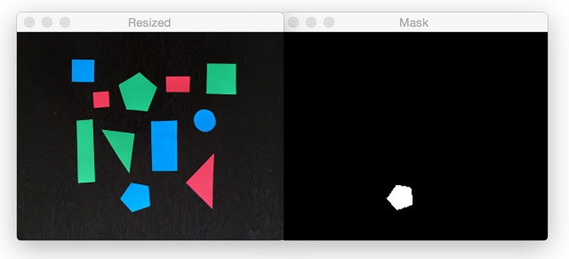
We’ll be processing a video streaming and looking for occurrences of this green ball:

Figure 1: An example of the green ball we are going to detect in video streams.

Figure 1: An example of the green ball we are going to detect in video streams.

If this green ball appears in our video stream, we’ll open up a new file video (based on the timestamp of occurrence), write the clip to file, and then stop the writing process once the ball disappears from our view.

Furthermore, our implementation will have a number of desirable properties, including:

  1. Writing frames to our video file a few seconds before the action takes place.
  2. Writing frames to file a few seconds after the action finishes — in both cases, our goal is to not only capture the entire event, but also the context of the event as well.
  3. Utilizing threads to ensure our main program is not slowed down when performing I/O on both the input stream and the output video clip file.
  4. Leveraging built-in Python data structures such as
    deque
      and
    Queue
      so we need not rely on external libraries (other than OpenCV and imutils, of course).

Project structure

Before we get started implementing our key event video writer, let’s look at the project structure:

|--- output
|--- pyimagesearch
|    |--- __init__.py
|    |--- keyclipwriter.py
|--- save_key_events.py

Inside the

pyimagesearch
  module, we’ll define a class named
KeyClipWriter
  inside the
keyclipwriter.py
  file. This class will handle accepting frames from an input video stream ad writing them to file in a safe, efficient, and threaded manner.

The driver script,

save_key_events.py
 , will define the criteria of what an “interesting event” is (i.e., the green ball entering the view of the camera), followed by passing these frames on to the
KeyClipWriter
  which will then create our video synopsis.

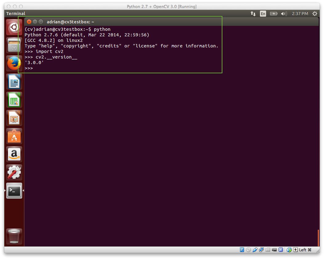
A quick note on Python + OpenCV versions

This blog post assumes you are using Python 3+ and OpenCV 3. As I mentioned in last week’s post, I wasn’t able to get the

cv2.VideoWriter
  function to work on my OpenCV 2.4 installation, so after a few hours of hacking around with no luck, I ended up abandoning OpenCV 2.4 for this project and sticking with OpenCV 3.

The code in this lesson is technically compatible with Python 2.7 (again, provided you are using Python 2.7 with OpenCV 3 bindings), but you’ll need to change a few

import
  statements (I’ll point these out along the way).

Writing key/interesting video clips to file with OpenCV

Let’s go ahead and get started reviewing our

KeyClipWriter
  class:
# import the necessary packages
from collections import deque
from threading import Thread
from queue import Queue
import time
import cv2

class KeyClipWriter:
	def __init__(self, bufSize=64, timeout=1.0):
		# store the maximum buffer size of frames to be kept
		# in memory along with the sleep timeout during threading
		self.bufSize = bufSize
		self.timeout = timeout

		# initialize the buffer of frames, queue of frames that
		# need to be written to file, video writer, writer thread,
		# and boolean indicating whether recording has started or not
		self.frames = deque(maxlen=bufSize)
		self.Q = None
		self.writer = None
		self.thread = None
		self.recording = False

We start off by importing our required Python packages on Lines 2-6. This tutorial assumes you are using Python 3, so if you’re using Python 2.7, you’ll need to change Line 4 from

from queue import Queue
  to simply
import Queue
 .

Line 9 defines the constructor to our

KeyClipWriter
 , which accepts two optional parameters:
  • bufSize
     : The maximum number of frames to be keep cached in an in-memory buffer.
  • timeout
     : An integer representing the number of seconds to sleep for when (1) writing video clips to file and (2) there are no frames ready to be written.

We then initialize four important variables on Lines 18-22:

  • frames
     : A buffer used to a store a maximum of
    bufSize
      frames that have been most recently read from the video stream.
  • Q
     : A “first in, first out” (FIFO) Python Queue data structure used to hold frames that are awaiting to be written to video file.
  • writer
     : An instantiation of the
    cv2.VideoWriter
      class used to actually write frames to the output video file.
  • thread
     : A Python
    Thread
      instance that we’ll use when writing videos to file (to avoid costly I/O latency delays).
  • recording
     : Boolean value indicating whether or not we are in “recording mode”.

Next up, let’s review the

update
  method:
# import the necessary packages
from collections import deque
from threading import Thread
from queue import Queue
import time
import cv2

class KeyClipWriter:
	def __init__(self, bufSize=64, timeout=1.0):
		# store the maximum buffer size of frames to be kept
		# in memory along with the sleep timeout during threading
		self.bufSize = bufSize
		self.timeout = timeout

		# initialize the buffer of frames, queue of frames that
		# need to be written to file, video writer, writer thread,
		# and boolean indicating whether recording has started or not
		self.frames = deque(maxlen=bufSize)
		self.Q = None
		self.writer = None
		self.thread = None
		self.recording = False

	def update(self, frame):
		# update the frames buffer
		self.frames.appendleft(frame)

		# if we are recording, update the queue as well
		if self.recording:
			self.Q.put(frame)

The

update
  function requires a single parameter, the
frame
  read from our video stream. We take this
frame
  and store it in our
frames
  buffer (Line 26). And if we are already in recording mode, we’ll store the
frame
  in the
Queue
  as well so it can be flushed to video file (Lines 29 and 30).

In order to kick-off an actual video clip recording, we need a

start
  method:
# import the necessary packages
from collections import deque
from threading import Thread
from queue import Queue
import time
import cv2

class KeyClipWriter:
	def __init__(self, bufSize=64, timeout=1.0):
		# store the maximum buffer size of frames to be kept
		# in memory along with the sleep timeout during threading
		self.bufSize = bufSize
		self.timeout = timeout

		# initialize the buffer of frames, queue of frames that
		# need to be written to file, video writer, writer thread,
		# and boolean indicating whether recording has started or not
		self.frames = deque(maxlen=bufSize)
		self.Q = None
		self.writer = None
		self.thread = None
		self.recording = False

	def update(self, frame):
		# update the frames buffer
		self.frames.appendleft(frame)

		# if we are recording, update the queue as well
		if self.recording:
			self.Q.put(frame)

	def start(self, outputPath, fourcc, fps):
		# indicate that we are recording, start the video writer,
		# and initialize the queue of frames that need to be written
		# to the video file
		self.recording = True
		self.writer = cv2.VideoWriter(outputPath, fourcc, fps,
			(self.frames[0].shape[1], self.frames[0].shape[0]), True)
		self.Q = Queue()

		# loop over the frames in the deque structure and add them
		# to the queue
		for i in range(len(self.frames), 0, -1):
			self.Q.put(self.frames[i - 1])

		# start a thread write frames to the video file
		self.thread = Thread(target=self.write, args=())
		self.thread.daemon = True
		self.thread.start()

First, we update our

recording
  boolean to indicate that we are in “recording mode”. Then, we initialize the
cv2.VideoWriter
  using the supplied
outputPath
 ,
fourcc
 , and
fps
  provided to the
start
  method, along with the frame spatial dimensions (i.e., width and height). For a complete review of the
cv2.VideoWriter
  parameters, please refer to this blog post.

Line 39 initializes our

Queue
  used to store the frames ready to be written to file. We then loop over all frames in our
frames
  buffer and add them to the queue.

Finally, we spawn a separate thread to handle writing frames to video — this way we don’t slow down our main video processing pipeline by waiting for I/O operations to complete.

As noted above, the

start
  method creates a new thread, calling the
write
  method used to write frames inside the
Q
  to file. Let’s define this
write
  method:
# import the necessary packages
from collections import deque
from threading import Thread
from queue import Queue
import time
import cv2

class KeyClipWriter:
	def __init__(self, bufSize=64, timeout=1.0):
		# store the maximum buffer size of frames to be kept
		# in memory along with the sleep timeout during threading
		self.bufSize = bufSize
		self.timeout = timeout

		# initialize the buffer of frames, queue of frames that
		# need to be written to file, video writer, writer thread,
		# and boolean indicating whether recording has started or not
		self.frames = deque(maxlen=bufSize)
		self.Q = None
		self.writer = None
		self.thread = None
		self.recording = False

	def update(self, frame):
		# update the frames buffer
		self.frames.appendleft(frame)

		# if we are recording, update the queue as well
		if self.recording:
			self.Q.put(frame)

	def start(self, outputPath, fourcc, fps):
		# indicate that we are recording, start the video writer,
		# and initialize the queue of frames that need to be written
		# to the video file
		self.recording = True
		self.writer = cv2.VideoWriter(outputPath, fourcc, fps,
			(self.frames[0].shape[1], self.frames[0].shape[0]), True)
		self.Q = Queue()

		# loop over the frames in the deque structure and add them
		# to the queue
		for i in range(len(self.frames), 0, -1):
			self.Q.put(self.frames[i - 1])

		# start a thread write frames to the video file
		self.thread = Thread(target=self.write, args=())
		self.thread.daemon = True
		self.thread.start()

	def write(self):
		# keep looping
		while True:
			# if we are done recording, exit the thread
			if not self.recording:
				return

			# check to see if there are entries in the queue
			if not self.Q.empty():
				# grab the next frame in the queue and write it
				# to the video file
				frame = self.Q.get()
				self.writer.write(frame)

			# otherwise, the queue is empty, so sleep for a bit
			# so we don't waste CPU cycles
			else:
				time.sleep(self.timeout)

Line 53 starts an infinite loop that will continue polling for new frames and writing them to file until our video recording has finished.

Lines 55 and 56 make a check to see if the recording should be stopped, and if so, we return from the thread.

Otherwise, if the

Q
  is not empty, we grab the next frame and write it to the video file (Lines 59-63).

If there are no frames in the

Q
 , we sleep for a bit so we don’t needlessly waste CPU cycles spinning (Lines 67 and 68). This is especially important when using the
Queue
  data structure which is thread-safe, implying that we must acquire a lock/semaphore prior to updating the internal buffer. If we don’t call
time.sleep
  when the buffer is empty, then the
write
  and
update
  methods will constantly be fighting for the lock. Instead, it’s best to let the writer sleep for a bit until there are a backlog of frames in the queue that need to be written to file.

We’ll also define a

flush
  method which simply takes all frames left in the
Q
  and dumps them to file:
# import the necessary packages
from collections import deque
from threading import Thread
from queue import Queue
import time
import cv2

class KeyClipWriter:
	def __init__(self, bufSize=64, timeout=1.0):
		# store the maximum buffer size of frames to be kept
		# in memory along with the sleep timeout during threading
		self.bufSize = bufSize
		self.timeout = timeout

		# initialize the buffer of frames, queue of frames that
		# need to be written to file, video writer, writer thread,
		# and boolean indicating whether recording has started or not
		self.frames = deque(maxlen=bufSize)
		self.Q = None
		self.writer = None
		self.thread = None
		self.recording = False

	def update(self, frame):
		# update the frames buffer
		self.frames.appendleft(frame)

		# if we are recording, update the queue as well
		if self.recording:
			self.Q.put(frame)

	def start(self, outputPath, fourcc, fps):
		# indicate that we are recording, start the video writer,
		# and initialize the queue of frames that need to be written
		# to the video file
		self.recording = True
		self.writer = cv2.VideoWriter(outputPath, fourcc, fps,
			(self.frames[0].shape[1], self.frames[0].shape[0]), True)
		self.Q = Queue()

		# loop over the frames in the deque structure and add them
		# to the queue
		for i in range(len(self.frames), 0, -1):
			self.Q.put(self.frames[i - 1])

		# start a thread write frames to the video file
		self.thread = Thread(target=self.write, args=())
		self.thread.daemon = True
		self.thread.start()

	def write(self):
		# keep looping
		while True:
			# if we are done recording, exit the thread
			if not self.recording:
				return

			# check to see if there are entries in the queue
			if not self.Q.empty():
				# grab the next frame in the queue and write it
				# to the video file
				frame = self.Q.get()
				self.writer.write(frame)

			# otherwise, the queue is empty, so sleep for a bit
			# so we don't waste CPU cycles
			else:
				time.sleep(self.timeout)

	def flush(self):
		# empty the queue by flushing all remaining frames to file
		while not self.Q.empty():
			frame = self.Q.get()
			self.writer.write(frame)

A method like this is used when a video recording has finished and we need to immediately flush all frames to file.

Finally, we define the

finish
  method below:
# import the necessary packages
from collections import deque
from threading import Thread
from queue import Queue
import time
import cv2

class KeyClipWriter:
	def __init__(self, bufSize=64, timeout=1.0):
		# store the maximum buffer size of frames to be kept
		# in memory along with the sleep timeout during threading
		self.bufSize = bufSize
		self.timeout = timeout

		# initialize the buffer of frames, queue of frames that
		# need to be written to file, video writer, writer thread,
		# and boolean indicating whether recording has started or not
		self.frames = deque(maxlen=bufSize)
		self.Q = None
		self.writer = None
		self.thread = None
		self.recording = False

	def update(self, frame):
		# update the frames buffer
		self.frames.appendleft(frame)

		# if we are recording, update the queue as well
		if self.recording:
			self.Q.put(frame)

	def start(self, outputPath, fourcc, fps):
		# indicate that we are recording, start the video writer,
		# and initialize the queue of frames that need to be written
		# to the video file
		self.recording = True
		self.writer = cv2.VideoWriter(outputPath, fourcc, fps,
			(self.frames[0].shape[1], self.frames[0].shape[0]), True)
		self.Q = Queue()

		# loop over the frames in the deque structure and add them
		# to the queue
		for i in range(len(self.frames), 0, -1):
			self.Q.put(self.frames[i - 1])

		# start a thread write frames to the video file
		self.thread = Thread(target=self.write, args=())
		self.thread.daemon = True
		self.thread.start()

	def write(self):
		# keep looping
		while True:
			# if we are done recording, exit the thread
			if not self.recording:
				return

			# check to see if there are entries in the queue
			if not self.Q.empty():
				# grab the next frame in the queue and write it
				# to the video file
				frame = self.Q.get()
				self.writer.write(frame)

			# otherwise, the queue is empty, so sleep for a bit
			# so we don't waste CPU cycles
			else:
				time.sleep(self.timeout)

	def flush(self):
		# empty the queue by flushing all remaining frames to file
		while not self.Q.empty():
			frame = self.Q.get()
			self.writer.write(frame)

	def finish(self):
		# indicate that we are done recording, join the thread,
		# flush all remaining frames in the queue to file, and
		# release the writer pointer
		self.recording = False
		self.thread.join()
		self.flush()
		self.writer.release()

This method indicates that the recording has been completed, joins the writer thread with the main script, flushes the remaining frames in the

Q
 to file, and finally releases the
cv2.VideoWriter
  pointer.

Now that we have defined the

KeyClipWriter
  class, we can move on to the driver script used to implement the “key/interesting event” detection.

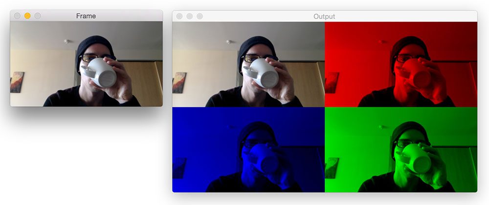
Saving key events with OpenCV

In order to keep this blog post simple and hands-on, we’ll define our “key event” to be when this green ball enters our video stream:

Figure 2: An example of a key/interesting event in a video stream.

Figure 2: An example of a key/interesting event in a video stream.

Once we see this green ball, we will call

KeyClipWriter
  to write all frames that contain the green ball to file. Essentially, this will give us a set of short video clips that neatly summarizes the events of the entire video stream — in short, a video synopsis.

Of course, you can use this code as a boilerplate/starting point to defining your own actions — we’ll simply use the “green ball” event since we have covered it multiple times before on the PyImageSearch blog, including tracking object movement and ball tracking.

Before you proceed with the rest of this tutorial, make sure you have the imutils package installed on your system:

$ pip install imutils

This will ensure that you can use the

VideoStream
  class which creates a unified access to both builtin/USB webcams and the Raspberry Pi camera module.

Let’s go ahead and get started. Open up the

save_key_events.py
  file and insert the following code:
# import the necessary packages
from pyimagesearch.keyclipwriter import KeyClipWriter
from imutils.video import VideoStream
import argparse
import datetime
import imutils
import time
import cv2

# construct the argument parse and parse the arguments
ap = argparse.ArgumentParser()
ap.add_argument("-o", "--output", required=True,
	help="path to output directory")
ap.add_argument("-p", "--picamera", type=int, default=-1,
	help="whether or not the Raspberry Pi camera should be used")
ap.add_argument("-f", "--fps", type=int, default=20,
	help="FPS of output video")
ap.add_argument("-c", "--codec", type=str, default="MJPG",
	help="codec of output video")
ap.add_argument("-b", "--buffer-size", type=int, default=32,
	help="buffer size of video clip writer")
args = vars(ap.parse_args())

Lines 2-8 import our necessary Python packages while Lines 11-22 parse our command line arguments. The set of command line arguments are detailed below:

  • --output
     : This is the path to the output directory where we will store the output video clips.
  • --picamera
     : If you want to use your Raspberry Pi camera (rather than a builtin/USB webcam), then supply a value of
    --picamera 1
     . You can read more about accessing both builtin/USB webcams and the Raspberry Pi camera module (without changing a single line of code) in this post.
  • --fps
     : This switch controls the desired FPS of your output video. This value should be similar to the number of frames per second your image processing pipeline can process.
  • --codec
     : The FourCC codec of the output video clips. Please see the previous post for more information.
  • --buffer-size
     : The size of the in-memory buffer used to store the most recently polled frames from the camera sensor. A larger
    --buffer-size
      will allow for more context before and after the “key event” to be included in the output video clip, while a smaller
    --buffer-size
      will store less frames before and after the “key event”.

Let’s perform some initialization:

# import the necessary packages
from pyimagesearch.keyclipwriter import KeyClipWriter
from imutils.video import VideoStream
import argparse
import datetime
import imutils
import time
import cv2

# construct the argument parse and parse the arguments
ap = argparse.ArgumentParser()
ap.add_argument("-o", "--output", required=True,
	help="path to output directory")
ap.add_argument("-p", "--picamera", type=int, default=-1,
	help="whether or not the Raspberry Pi camera should be used")
ap.add_argument("-f", "--fps", type=int, default=20,
	help="FPS of output video")
ap.add_argument("-c", "--codec", type=str, default="MJPG",
	help="codec of output video")
ap.add_argument("-b", "--buffer-size", type=int, default=32,
	help="buffer size of video clip writer")
args = vars(ap.parse_args())

# initialize the video stream and allow the camera sensor to
# warmup
print("[INFO] warming up camera...")
vs = VideoStream(usePiCamera=args["picamera"] > 0).start()
time.sleep(2.0)

# define the lower and upper boundaries of the "green" ball in
# the HSV color space
greenLower = (29, 86, 6)
greenUpper = (64, 255, 255)

# initialize key clip writer and the consecutive number of
# frames that have *not* contained any action
kcw = KeyClipWriter(bufSize=args["buffer_size"])
consecFrames = 0

Lines 26-28 initialize our

VideoStream
  and allow the camera sensor to warmup.

From there, Lines 32 and 33 define the lower and upper color threshold boundaries for the green ball in the HSV color space. For more information on how we defined these color threshold values, please see this post.

Line 37 instantiates our

KeyClipWriter
  using our supplied
--buffer-size
 , along with initializing an integer used to count the number of consecutive frames that have not contained any interesting events.

We are now ready to start processing frames from our video stream:

# import the necessary packages
from pyimagesearch.keyclipwriter import KeyClipWriter
from imutils.video import VideoStream
import argparse
import datetime
import imutils
import time
import cv2

# construct the argument parse and parse the arguments
ap = argparse.ArgumentParser()
ap.add_argument("-o", "--output", required=True,
	help="path to output directory")
ap.add_argument("-p", "--picamera", type=int, default=-1,
	help="whether or not the Raspberry Pi camera should be used")
ap.add_argument("-f", "--fps", type=int, default=20,
	help="FPS of output video")
ap.add_argument("-c", "--codec", type=str, default="MJPG",
	help="codec of output video")
ap.add_argument("-b", "--buffer-size", type=int, default=32,
	help="buffer size of video clip writer")
args = vars(ap.parse_args())

# initialize the video stream and allow the camera sensor to
# warmup
print("[INFO] warming up camera...")
vs = VideoStream(usePiCamera=args["picamera"] > 0).start()
time.sleep(2.0)

# define the lower and upper boundaries of the "green" ball in
# the HSV color space
greenLower = (29, 86, 6)
greenUpper = (64, 255, 255)

# initialize key clip writer and the consecutive number of
# frames that have *not* contained any action
kcw = KeyClipWriter(bufSize=args["buffer_size"])
consecFrames = 0

# keep looping
while True:
	# grab the current frame, resize it, and initialize a
	# boolean used to indicate if the consecutive frames
	# counter should be updated
	frame = vs.read()
	frame = imutils.resize(frame, width=600)
	updateConsecFrames = True

	# blur the frame and convert it to the HSV color space
	blurred = cv2.GaussianBlur(frame, (11, 11), 0)
	hsv = cv2.cvtColor(blurred, cv2.COLOR_BGR2HSV)

	# construct a mask for the color "green", then perform
	# a series of dilations and erosions to remove any small
	# blobs left in the mask
	mask = cv2.inRange(hsv, greenLower, greenUpper)
	mask = cv2.erode(mask, None, iterations=2)
	mask = cv2.dilate(mask, None, iterations=2)

	# find contours in the mask
	cnts = cv2.findContours(mask.copy(), cv2.RETR_EXTERNAL,
		cv2.CHAIN_APPROX_SIMPLE)
	cnts = cnts[0] if imutils.is_cv2() else cnts[1]

On Line 41 we start to looping over frames from our video stream. Lines 45 and 46 read the next

frame
  from the video stream and then resizes it to have a width of 600 pixels.

Further pre-processing is done on Lines 50 and 51 by blurring the image slightly and then converting the image from the RGB color space to the HSV color space (so we can apply our color thresholding).

The actual color thresholding is performed on Line 56 using the

cv2.inRange
  function. This method finds all pixels p that are
greenLower <= p <= greenUpper
 . We then perform a series of erosions and dilations to remove any small blobs left in the mask.

Finally, Lines 61-63 find contours in the thresholded image.

If you are confused about any step of this processing pipeline, I would suggest going back to our previous posts on ball tracking and object movement to further familiarize yourself with the topic.

We are now ready to check and see if the green ball was found in our image:

# import the necessary packages
from pyimagesearch.keyclipwriter import KeyClipWriter
from imutils.video import VideoStream
import argparse
import datetime
import imutils
import time
import cv2

# construct the argument parse and parse the arguments
ap = argparse.ArgumentParser()
ap.add_argument("-o", "--output", required=True,
	help="path to output directory")
ap.add_argument("-p", "--picamera", type=int, default=-1,
	help="whether or not the Raspberry Pi camera should be used")
ap.add_argument("-f", "--fps", type=int, default=20,
	help="FPS of output video")
ap.add_argument("-c", "--codec", type=str, default="MJPG",
	help="codec of output video")
ap.add_argument("-b", "--buffer-size", type=int, default=32,
	help="buffer size of video clip writer")
args = vars(ap.parse_args())

# initialize the video stream and allow the camera sensor to
# warmup
print("[INFO] warming up camera...")
vs = VideoStream(usePiCamera=args["picamera"] > 0).start()
time.sleep(2.0)

# define the lower and upper boundaries of the "green" ball in
# the HSV color space
greenLower = (29, 86, 6)
greenUpper = (64, 255, 255)

# initialize key clip writer and the consecutive number of
# frames that have *not* contained any action
kcw = KeyClipWriter(bufSize=args["buffer_size"])
consecFrames = 0

# keep looping
while True:
	# grab the current frame, resize it, and initialize a
	# boolean used to indicate if the consecutive frames
	# counter should be updated
	frame = vs.read()
	frame = imutils.resize(frame, width=600)
	updateConsecFrames = True

	# blur the frame and convert it to the HSV color space
	blurred = cv2.GaussianBlur(frame, (11, 11), 0)
	hsv = cv2.cvtColor(blurred, cv2.COLOR_BGR2HSV)

	# construct a mask for the color "green", then perform
	# a series of dilations and erosions to remove any small
	# blobs left in the mask
	mask = cv2.inRange(hsv, greenLower, greenUpper)
	mask = cv2.erode(mask, None, iterations=2)
	mask = cv2.dilate(mask, None, iterations=2)

	# find contours in the mask
	cnts = cv2.findContours(mask.copy(), cv2.RETR_EXTERNAL,
		cv2.CHAIN_APPROX_SIMPLE)
	cnts = cnts[0] if imutils.is_cv2() else cnts[1]

	# only proceed if at least one contour was found
	if len(cnts) > 0:
		# find the largest contour in the mask, then use it
		# to compute the minimum enclosing circle
		c = max(cnts, key=cv2.contourArea)
		((x, y), radius) = cv2.minEnclosingCircle(c)
		updateConsecFrames = radius <= 10

		# only proceed if the redius meets a minimum size
		if radius > 10:
			# reset the number of consecutive frames with
			# *no* action to zero and draw the circle
			# surrounding the object
			consecFrames = 0
			cv2.circle(frame, (int(x), int(y)), int(radius),
				(0, 0, 255), 2)

			# if we are not already recording, start recording
			if not kcw.recording:
				timestamp = datetime.datetime.now()
				p = "{}/{}.avi".format(args["output"],
					timestamp.strftime("%Y%m%d-%H%M%S"))
				kcw.start(p, cv2.VideoWriter_fourcc(*args["codec"]),
					args["fps"])

Line 66 makes a check to ensure that at least one contour was found, and if so, Line 69 and 70 find the largest contour in the mask (according to the area) and use this contour to compute the minimum enclosing circle.

If the radius of the circle meets a minimum suze of 10 pixels (Line 74), then we will assume that we have found the green ball. Lines 78-80 reset the number of

consecFrames
  that do not contain any interesting events (since an interesting event is “currently happening”) and draw a circle highlighting our ball in the frame.

Finally, we make a check if to see if we are currently recording a video clip (Line 83). If not, we generate an output filename for the video clip based on the current timestamp and call the

start
  method of the
KeyClipWriter
 .

Otherwise, we’ll assume no key/interesting event has taken place:

# import the necessary packages
from pyimagesearch.keyclipwriter import KeyClipWriter
from imutils.video import VideoStream
import argparse
import datetime
import imutils
import time
import cv2

# construct the argument parse and parse the arguments
ap = argparse.ArgumentParser()
ap.add_argument("-o", "--output", required=True,
	help="path to output directory")
ap.add_argument("-p", "--picamera", type=int, default=-1,
	help="whether or not the Raspberry Pi camera should be used")
ap.add_argument("-f", "--fps", type=int, default=20,
	help="FPS of output video")
ap.add_argument("-c", "--codec", type=str, default="MJPG",
	help="codec of output video")
ap.add_argument("-b", "--buffer-size", type=int, default=32,
	help="buffer size of video clip writer")
args = vars(ap.parse_args())

# initialize the video stream and allow the camera sensor to
# warmup
print("[INFO] warming up camera...")
vs = VideoStream(usePiCamera=args["picamera"] > 0).start()
time.sleep(2.0)

# define the lower and upper boundaries of the "green" ball in
# the HSV color space
greenLower = (29, 86, 6)
greenUpper = (64, 255, 255)

# initialize key clip writer and the consecutive number of
# frames that have *not* contained any action
kcw = KeyClipWriter(bufSize=args["buffer_size"])
consecFrames = 0

# keep looping
while True:
	# grab the current frame, resize it, and initialize a
	# boolean used to indicate if the consecutive frames
	# counter should be updated
	frame = vs.read()
	frame = imutils.resize(frame, width=600)
	updateConsecFrames = True

	# blur the frame and convert it to the HSV color space
	blurred = cv2.GaussianBlur(frame, (11, 11), 0)
	hsv = cv2.cvtColor(blurred, cv2.COLOR_BGR2HSV)

	# construct a mask for the color "green", then perform
	# a series of dilations and erosions to remove any small
	# blobs left in the mask
	mask = cv2.inRange(hsv, greenLower, greenUpper)
	mask = cv2.erode(mask, None, iterations=2)
	mask = cv2.dilate(mask, None, iterations=2)

	# find contours in the mask
	cnts = cv2.findContours(mask.copy(), cv2.RETR_EXTERNAL,
		cv2.CHAIN_APPROX_SIMPLE)
	cnts = cnts[0] if imutils.is_cv2() else cnts[1]

	# only proceed if at least one contour was found
	if len(cnts) > 0:
		# find the largest contour in the mask, then use it
		# to compute the minimum enclosing circle
		c = max(cnts, key=cv2.contourArea)
		((x, y), radius) = cv2.minEnclosingCircle(c)
		updateConsecFrames = radius <= 10

		# only proceed if the redius meets a minimum size
		if radius > 10:
			# reset the number of consecutive frames with
			# *no* action to zero and draw the circle
			# surrounding the object
			consecFrames = 0
			cv2.circle(frame, (int(x), int(y)), int(radius),
				(0, 0, 255), 2)

			# if we are not already recording, start recording
			if not kcw.recording:
				timestamp = datetime.datetime.now()
				p = "{}/{}.avi".format(args["output"],
					timestamp.strftime("%Y%m%d-%H%M%S"))
				kcw.start(p, cv2.VideoWriter_fourcc(*args["codec"]),
					args["fps"])

	# otherwise, no action has taken place in this frame, so
	# increment the number of consecutive frames that contain
	# no action
	if updateConsecFrames:
		consecFrames += 1

	# update the key frame clip buffer
	kcw.update(frame)

	# if we are recording and reached a threshold on consecutive
	# number of frames with no action, stop recording the clip
	if kcw.recording and consecFrames == args["buffer_size"]:
		kcw.finish()

	# show the frame
	cv2.imshow("Frame", frame)
	key = cv2.waitKey(1) & 0xFF

	# if the `q` key was pressed, break from the loop
	if key == ord("q"):
		break

If no interesting event has happened, we update

consecFrames
  and pass the
frame
  over to our buffer.

Line 101 makes an important check — if we are recording and have reached a sufficient number of consecutive frames with no key event, then we should stop the recording.

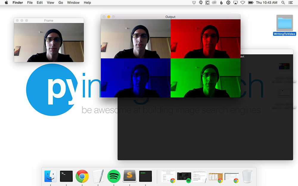
Finally, Lines 105-110 display the output

frame
  to our screen and wait for a keypress.

Our final block of code ensures the video has been successfully closed and then performs a bit of cleanup:

# import the necessary packages
from pyimagesearch.keyclipwriter import KeyClipWriter
from imutils.video import VideoStream
import argparse
import datetime
import imutils
import time
import cv2

# construct the argument parse and parse the arguments
ap = argparse.ArgumentParser()
ap.add_argument("-o", "--output", required=True,
	help="path to output directory")
ap.add_argument("-p", "--picamera", type=int, default=-1,
	help="whether or not the Raspberry Pi camera should be used")
ap.add_argument("-f", "--fps", type=int, default=20,
	help="FPS of output video")
ap.add_argument("-c", "--codec", type=str, default="MJPG",
	help="codec of output video")
ap.add_argument("-b", "--buffer-size", type=int, default=32,
	help="buffer size of video clip writer")
args = vars(ap.parse_args())

# initialize the video stream and allow the camera sensor to
# warmup
print("[INFO] warming up camera...")
vs = VideoStream(usePiCamera=args["picamera"] > 0).start()
time.sleep(2.0)

# define the lower and upper boundaries of the "green" ball in
# the HSV color space
greenLower = (29, 86, 6)
greenUpper = (64, 255, 255)

# initialize key clip writer and the consecutive number of
# frames that have *not* contained any action
kcw = KeyClipWriter(bufSize=args["buffer_size"])
consecFrames = 0

# keep looping
while True:
	# grab the current frame, resize it, and initialize a
	# boolean used to indicate if the consecutive frames
	# counter should be updated
	frame = vs.read()
	frame = imutils.resize(frame, width=600)
	updateConsecFrames = True

	# blur the frame and convert it to the HSV color space
	blurred = cv2.GaussianBlur(frame, (11, 11), 0)
	hsv = cv2.cvtColor(blurred, cv2.COLOR_BGR2HSV)

	# construct a mask for the color "green", then perform
	# a series of dilations and erosions to remove any small
	# blobs left in the mask
	mask = cv2.inRange(hsv, greenLower, greenUpper)
	mask = cv2.erode(mask, None, iterations=2)
	mask = cv2.dilate(mask, None, iterations=2)

	# find contours in the mask
	cnts = cv2.findContours(mask.copy(), cv2.RETR_EXTERNAL,
		cv2.CHAIN_APPROX_SIMPLE)
	cnts = cnts[0] if imutils.is_cv2() else cnts[1]

	# only proceed if at least one contour was found
	if len(cnts) > 0:
		# find the largest contour in the mask, then use it
		# to compute the minimum enclosing circle
		c = max(cnts, key=cv2.contourArea)
		((x, y), radius) = cv2.minEnclosingCircle(c)
		updateConsecFrames = radius <= 10

		# only proceed if the redius meets a minimum size
		if radius > 10:
			# reset the number of consecutive frames with
			# *no* action to zero and draw the circle
			# surrounding the object
			consecFrames = 0
			cv2.circle(frame, (int(x), int(y)), int(radius),
				(0, 0, 255), 2)

			# if we are not already recording, start recording
			if not kcw.recording:
				timestamp = datetime.datetime.now()
				p = "{}/{}.avi".format(args["output"],
					timestamp.strftime("%Y%m%d-%H%M%S"))
				kcw.start(p, cv2.VideoWriter_fourcc(*args["codec"]),
					args["fps"])

	# otherwise, no action has taken place in this frame, so
	# increment the number of consecutive frames that contain
	# no action
	if updateConsecFrames:
		consecFrames += 1

	# update the key frame clip buffer
	kcw.update(frame)

	# if we are recording and reached a threshold on consecutive
	# number of frames with no action, stop recording the clip
	if kcw.recording and consecFrames == args["buffer_size"]:
		kcw.finish()

	# show the frame
	cv2.imshow("Frame", frame)
	key = cv2.waitKey(1) & 0xFF

	# if the `q` key was pressed, break from the loop
	if key == ord("q"):
		break

# if we are in the middle of recording a clip, wrap it up
if kcw.recording:
	kcw.finish()

# do a bit of cleanup
cv2.destroyAllWindows()
vs.stop()

Video synopsis results

To generate video clips for key events (i.e., the green ball appearing on our video stream), just execute the following command:

$ python save_key_events.py --output output

I’ve included the full 1m 46s video (without extracting salient clips) below:
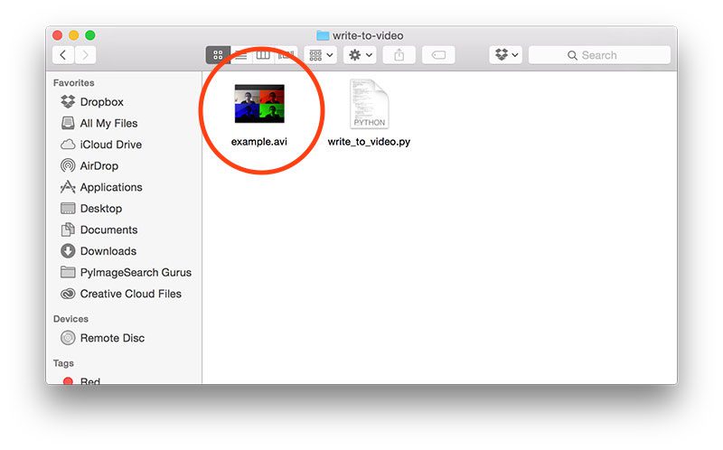
After running the

save_key_events.py
  script, I now have 4 output videos, one for each the time green ball was present in my video stream:
Figure 3: Creating a separate video clip for each interesting and key event.

Figure 3: Creating a separate video clip for each interesting and key event.

The key event video clips are displayed below to demonstrate that our script is working properly, accurately extracting our “interesting events”, and essentially building a series of video clips functioning as a video synopsis:

Video clip #1:

Video clip #2:

Video clip #3:

Video clip #4:

Summary

In this blog post, we learned how to save key event video clips to file using OpenCV and Python.

Exactly what defines a “key or interesting event” is entirely dependent on your application and the goals of your overall project. Examples of key events can include:

  • Monitoring your front door for motion detection (i.e., someone entering your house).
  • Recognizing the face of an intruder as they enter your house.
  • Reporting unsafe driving outside your home to the authorities.

Again, exactly what constitutes a “key event” is near endless. However, regardless of how you define an interesting event, you can still use the Python code detailed in this post to help save these interesting events to file as a shortened video clip.

Using this methodology, you can condense hours of video stream footage into seconds of interesting events, effectively yielding a video synopsis — all generated using Python, computer vision, and image processing techniques.

Anyway, I hope you enjoyed this blog post!

If you did, please consider sharing it on your favorite social media outlet such as Facebook, Twitter, LinkedIn, etc. I put a lot of effort into the past two blog posts in this series and I would really appreciate it if you could help spread the word.

And before you, be sure to signup for the PyImageSearch Newsletter using the form below to receive email updates when new posts go live!

Downloads:

If you would like to download the code and images used in this post, please enter your email address in the form below. Not only will you get a .zip of the code, I’ll also send you a FREE 11-page Resource Guide on Computer Vision and Image Search Engines, including exclusive techniques that I don’t post on this blog! Sound good? If so, enter your email address and I’ll send you the code immediately!

The post Saving key event video clips with OpenCV appeared first on PyImageSearch.

Install guide: Raspberry Pi 3 + Raspbian Jessie + OpenCV 3

$
0
0

rpi3_board

Can you believe it’s been over four years since the original Raspberry Pi model B was released? Back then the Pi Model B shipped with only 256MB of RAM and a 700MHz single core processor.

Just over one year ago the Raspberry Pi 2 was unleashed on the world. And man, for something called a “Pi”, this beast made an impact on the computer world like an asteroid. This board sported 1GB of RAM and a 900MHz quad-core processor — quite the upgrade from the original single core, 700MHz system!

In my opinion, the Raspberry Pi 2 is what made computer vision possible on the Pi platform (at least from a Python + OpenCV perspective). The original model B simply didn’t have the processing capacity (or the RAM) to be powerful enough to process images video streams for anything more than trivial operations — the Pi 2 changed all that.

In fact, the Raspberry Pi 2 had such a meaningful impact on the computer vision space, that I even took the time to make a all code examples in Practical Python and OpenCV compatible with the Pi.

And now we have the Raspberry Pi 3:

  • 1.2Ghz 64-bit quad-core processor.
  • 1GB RAM.
  • Integrated 802.11n wireless and bluetooth.

Personally, I was hoping for a bit more RAM (perhaps in the range of 1.5-2GB). But upgrading to a 64-bit processor with 33% increased performance is well worth it.

Just as I have done in previous blog posts, I’ll be demonstrating how to install OpenCV 3 with Python bindings on Raspbian Jessie.

If you are looking for previous installation instructions for different platforms, please consult this list:

Otherwise, let’s proceed with getting OpenCV 3 installed on your brand new Raspberry Pi 3!

Assumptions

In this tutorial, I am going to assume that you already own a Raspberry Pi 3 with Raspbian Jessie installed.

You should also have either:

  • Physical access to your Raspberry Pi 3 so that you can open up a terminal and execute commands.
  • Remote access via SSH.

I’ll be doing the majority of this tutorial via SSH, but as long as you have access to a terminal, you can easily follow along.

Installing OpenCV 3 on a Raspberry Pi 3 running Raspbian Jessie

If you’ve ever installed OpenCV on a Raspberry Pi (or any other platform before), you know that the process can be quite time consuming with many dependencies and pre-requisites that have to be installed. The goal of this tutorial is to thus guide you step-by-step through the compile and installation process.

In order to make the installation process go more smoothly, I’ve included timings for each step so you know when to take a break, grab a cup of coffee, and checkup on email while the Pi compiles OpenCV. That said, the Pi 3 is substantially faster than the Pi 2, so the time it takes to compile OpenCV has decreased dramatically.

Anyway, let’s go ahead and get started installing OpenCV 3 on your brand new Raspberry Pi 3 running Raspbian Jessie.

Step #1: Expand filesystem

Are you using a brand new install of Raspbian Jessie?

If so, the first thing you should do is expand your filesystem to include all available space on your micro-SD card:

$ sudo raspi-config

Figure 1: Expanding the filesystem on your Raspberry Pi 3.

Figure 1: Expanding the filesystem on your Raspberry Pi 3.

Once prompted, you should select the first option, “1. Expand File System”, hit Enter on your keyboard, arrow down to the “<Finish>” button, and then reboot your Pi:

$ sudo reboot

After rebooting, your file system should have been expanded to include all available space on your micro-SD card. You can verify that the disk has been expanded by executing

df -h
  and examining the output:
$ df -h
Filesystem      Size  Used Avail Use% Mounted on
/dev/root       7.2G  3.3G  3.6G  48% /
devtmpfs        459M     0  459M   0% /dev
tmpfs           463M     0  463M   0% /dev/shm
tmpfs           463M  6.4M  457M   2% /run
tmpfs           5.0M  4.0K  5.0M   1% /run/lock
tmpfs           463M     0  463M   0% /sys/fs/cgroup
/dev/mmcblk0p1   60M   20M   41M  34% /boot
tmpfs            93M     0   93M   0% /run/user/1000

As you can see, my Raspbian filesystem has been expanded to include all 8GB of the micro-SD card.

However, even with my filesystem expanded, I have already used 48% of my 8GB card!

OpenCV, along with all its dependencies, will need a few gigabytes during the compile, so you should delete the Wolfram engine to free up some space on your Pi:

$ sudo apt-get purge wolfram-engine

After removing the Wolfram Engine, you can reclaim almost 700mb!

Step #2: Install dependencies

This isn’t the first time I’ve discussed how to install OpenCV on the Raspberry Pi, so I’ll keep these instructions on the briefer side, allowing you to work through the installation process: I’ve also included the amount of time it takes to execute each command so you can plan your OpenCV + Raspberry Pi 3 install accordingly (OpenCV itself takes 1h 12m to compile).

The first step is to update and upgrade any existing packages:

$ sudo apt-get update
$ sudo apt-get upgrade

Timing: 1m 26s

We then need to install some developer tools, including CMake, which helps us configure the OpenCV build process:

$ sudo apt-get install build-essential cmake pkg-config

Timing: 40s

Next, we need to install some image I/O packages that allow us to load various image file formats from disk. Examples of such file formats include JPEG, PNG, TIFF, etc.:

$ sudo apt-get install libjpeg-dev libtiff5-dev libjasper-dev libpng12-dev

Timing: 32s

Just as we need image I/O packages, we also need video I/O packages. These libraries allow us to read various video file formats from disk as well as work directly with video streams:

$ sudo apt-get install libavcodec-dev libavformat-dev libswscale-dev libv4l-dev
$ sudo apt-get install libxvidcore-dev libx264-dev

Timing: 34s

The OpenCV library comes with a sub-module named

highgui
  which is used to display images to our screen and build basic GUIs. In order to compile the
highgui
  module, we need to install the GTK development library:
$ sudo apt-get install libgtk2.0-dev

Timing: 3m 6s

Many operations inside of OpenCV (namely matrix operations) can be optimized further by installing a few extra dependencies:

$ sudo apt-get install libatlas-base-dev gfortran

Timing: 46s

These optimization libraries are especially important for resource constrained devices such as the Raspberry Pi.

Lastly, let’s install both the Python 2.7 and Python 3 header files so we can compile OpenCV with Python bindings:

$ sudo apt-get install python2.7-dev python3-dev

Timing: 45s

If you skip this step, you may notice an error related to the

Python.h
  header file not being found when running
make
  to compile OpenCV.

Step #3: Download the OpenCV source code

Now that we have our dependencies installed, let’s grab the

3.1.0
  archive of OpenCV from the official OpenCV repository. (Note: As future versions of openCV are released, you can replace
3.1.0
  with the latest version number):
$ cd ~
$ wget -O opencv.zip https://github.com/Itseez/opencv/archive/3.1.0.zip
$ unzip opencv.zip

Timing: 1m 26s

We’ll want the full install of OpenCV 3 (to have access to features such as SIFT and SURF, for instance), so we also need to grab the opencv_contrib repository as well:

$ wget -O opencv_contrib.zip https://github.com/Itseez/opencv_contrib/archive/3.1.0.zip
$ unzip opencv_contrib.zip

Timing: 43s

You might need to expand the command above using the “<=>” button during your copy and paste. The

.zip
  in the
3.1.0.zip
  may appear to be cutoff in some browsers. The full URL of the OpenCV 3.1.0 archive is:

https://github.com/Itseez/opencv_contrib/archive/3.1.0.zip

Note: Make sure your

opencv
  and
opencv_contrib
  versions are the same (in this case,
3.1.0
 ). If the versions numbers do not match up, then you’ll likely run into either compile-time or runtime.

Step #4: Python 2.7 or Python 3?

Before we can start compiling OpenCV on our Raspberry Pi 3, we first need to install

pip
 , a Python package manager:
$ wget https://bootstrap.pypa.io/get-pip.py
$ sudo python get-pip.py

Timing: 20s

If you’re a longtime PyImageSearch reader, then you’ll know that I’m a huge fan of both virtualenv and virtualenvwrapper. Installing these packages is not a requirement and you can absolutely get OpenCV installed without them, but that said, I highly recommend you install them as other PyImageSearch tutorials in the future will also leverage Python virtual environments. I’ll also be assuming that you have both

virtualenv
  and
virtualenvwrapper
  installed throughout the remainder of this guide.

So, given that, what’s the point of using

virtualenv
  and
virtualenvwrapper
 ?

First, it’s important to understand that a virtual environment is a special tool used to keep the dependencies required by different projects in separate places by creating isolated, independent Python environments for each of them.

In short, it solves the “Project X depends on version 1.x, but Project Y needs 4.x” dilemma. It also keeps your global

site-packages
  neat, tidy, and free from clutter.

If you would like a full explanation on why Python virtual environments are good practice, absolutely give this excellent blog post on RealPython a read.

It’s standard practice in the Python community to be using virtual environments of some sort, so I highly recommend that you do the same:

$ sudo pip install virtualenv virtualenvwrapper
$ sudo rm -rf ~/.cache/pip

Timing: 9s

Now that both

virtualenv
  and
virtualenvwrapper
  have been installed, we need to update our
~/.profile
  file to include the following lines at the bottom of the file:
# virtualenv and virtualenvwrapper
export WORKON_HOME=$HOME/.virtualenvs
source /usr/local/bin/virtualenvwrapper.sh

In previous tutorials, I’ve recommended using your favorite terminal-based text editor such as

vim
 ,
emacs
 , or
nano
  to update the
~/.profile
  file. If you’re comfortable with these editors, go ahead and update the file to reflect the changes mentioned above.

Otherwise, you should simply use

cat
  and output redirection to handle updating
~/.profile
 :
$ echo -e "\n# virtualenv and virtualenvwrapper" >> ~/.profile
$ echo "export WORKON_HOME=$HOME/.virtualenvs" >> ~/.profile
$ echo "source /usr/local/bin/virtualenvwrapper.sh" >> ~/.profile

Now that we have our

~/.profile
  updated, we need to reload it to make sure the changes take affect. You can force a reload of your
~/.profile
  file by:
  1. Logging out and then logging back in.
  2. Closing a terminal instance and opening up a new one
  3. Oor my personal favorite, just use the
    source
      command:

$ source ~/.profile

Note: I recommend running the

source ~/.profile
  file each time you open up a new terminal to ensure your system variables have been setup correctly.

Creating your Python virtual environment

Next, let’s create the Python virtual environment that we’ll use for computer vision development:

$ mkvirtualenv cv -p python2

This command will create a new Python virtual environment named

cv
  using Python 2.7.

If you instead want to use Python 3, you’ll want to use this command instead:

$ mkvirtualenv cv -p python3

Again, I can’t stress this point enough: the

cv
  Python virtual environment is entirely independent and sequestered from the default Python version included in the download of Raspbian Jessie. Any Python packages in the global
site-packages
  directory will not be available to the
cv
  virtual environment. Similarly, any Python packages installed in
site-packages
  of
cv
  will not be available to the global install of Python. Keep this in mind when you’re working in your Python virtual environment and it will help avoid a lot of confusion and headaches.

How to check if you’re in the “cv” virtual environment

If you ever reboot your Raspberry Pi; log out and log back in; or open up a new terminal, you’ll need to use the

workon
  command to re-access the
cv
  virtual environment. In previous blog posts, I’ve seen readers use the
mkvirtualenv
  command — this is entirely unneeded! The
mkvirtualenv
  command is meant to be executed only once: to actually create the virtual environment.

After that, you can use

workon
  and you’ll be dropped down into your virtual environment:
$ source ~/.profile
$ workon cv

To validate and ensure you are in the

cv
  virtual environment, examine your command line — if you see the text
(cv)
  preceding your prompt, then you are in the
cv
  virtual environment:
Figure 2: Make sure you see the "(cv)" text on your prompt, indicating that you are in the cv virtual environment.

Figure 2: Make sure you see the “(cv)” text on your prompt, indicating that you are in the cv virtual environment.

Otherwise, if you do not see the

(cv)
  text, then you are not in the
cv
  virtual environment:
Figure 3: If you do not see the "(cv)" text on your prompt, then you are not in the cv virtual environment and need to run "source" and "workon" to resolve this issue.

Figure 3: If you do not see the “(cv)” text on your prompt, then you are not in the cv virtual environment and need to run “source” and “workon” to resolve this issue.

To fix this, simply execute the

source
  and
workon
  commands mentioned above.

Installing NumPy on your Raspberry Pi

Assuming you’ve made it this far, you should now be in the

cv
  virtual environment (which you should stay in for the rest of this tutorial). Our only Python dependency is NumPy, a Python package used for numerical processing:
$ pip install numpy

Timing: 9m 39s

Be sure to grab a cup of coffee or go for a nice walk, the NumPy installation can take a bit of time.

Note: Another question I’ve often seen is “Help, my NumPy installation has hung and it’s not installing!” Actually, it is installing, it just takes time to pull down the sources and compile. Be patient. The Raspberry Pi isn’t as fast as your laptop/desktop.

Step #5: Compile and Install OpenCV

We are now ready to compile and install OpenCV! Double-check that you are in the

cv
  virtual environment by examining your prompt (you should see the
(cv)
  text preceding it), and if not, simply execute
workon
 :
$ workon cv

Once you have ensured you are in the

cv
  virtual environment, we can setup our build using CMake:
$ cd ~/opencv-3.1.0/
$ mkdir build
$ cd build
$ cmake -D CMAKE_BUILD_TYPE=RELEASE \
    -D CMAKE_INSTALL_PREFIX=/usr/local \
    -D INSTALL_PYTHON_EXAMPLES=ON \
    -D OPENCV_EXTRA_MODULES_PATH=~/opencv_contrib-3.1.0/modules \
    -D BUILD_EXAMPLES=ON ..

Timing: 1m 57s

Now, before we move on to the actual compilation step, make sure you examine the output of CMake!

Start by scrolling down the section titled

Python 2
  and
Python 3
 .

If you are compiling OpenCV 3 for Python 2.7, then make sure your

Python 2
  section includes valid paths to the
Interpreter
 ,
Libraries
 ,
numpy
  and
packages path
 , similar to my screenshot below:
Figure 4: Ensuring that Python 2.7 will be used when compiling OpenCV 3 for Raspbian Jessie on the Raspberry Pi 3.

Figure 4: Ensuring that Python 2.7 will be used when compiling OpenCV 3 for Raspbian Jessie on the Raspberry Pi 3.

Notice how the

Interpreter
  points to our
python2.7
  binary located in the
cv
  virtual environment. The
numpy
  variable also points to the NumPy installation in the
cv
  environment.

Similarly, if you’re compiling OpenCV for Python 3, make sure the

Python 3
  section looks like the figure below:
Figure 5: Checking that Python 3 will be used when compiling OpenCV 3 for Raspbian Jessie on the Raspberry Pi 3.

Figure 5: Checking that Python 3 will be used when compiling OpenCV 3 for Raspbian Jessie on the Raspberry Pi 3.

Again, the

Interpreter
  points to our
python3.4
  binary located in the
cv
  virtual environment while
numpy
  points to our NumPy install.

In either case, if you do not see the

cv
  virtual environment in these variables paths, it’s almost certainly because you are NOT in the
cv
  virtual environment prior to running CMake! 

If this is the case, access the

cv
  virtual environment using
workon cv
  and re-run the
cmake
  command outlined above.

Finally, we are now ready to compile OpenCV:

$ make -j4

Timing: 1h 12m

Note: Compiling OpenCV in 72 minutes on the Raspberry Pi 3 is a 24% improvement over the previous 95 minutes for the Raspberry Pi 2. That extra 300MHz makes a big difference!

The

-j4
  command controls the number of cores to leverage when compiling OpenCV 3. The Raspberry Pi 3 has four cores, thus we supply a value of
4
  to allow OpenCV to compile faster.

However, due to race conditions, there are times when

make
  errors out when using multiple cores. If this happens to you, I suggest starting the compilation over again and using only one core:
$ make clean
$ make

Once OpenCV 3 has finished compiling, your output should look similar to mine below:

Figure 5: Our OpenCV 3 compile on Raspbian Jessie has completed successfully.

Figure 5: Our OpenCV 3 compile on Raspbian Jessie has completed successfully.

From there, all you need to do is install OpenCV 3 on your Raspberry Pi 3:

$ sudo make install
$ sudo ldconfig

Timing: 52s

Step #6: Finish installing OpenCV on your Pi

We’re almost done — just a few more steps to go and you’ll be ready to use your Raspberry Pi 3 with OpenCV 3.

For Python 2.7:

Provided your Step #5 finished without error, OpenCV should now be installed in

/usr/local/lib/python2.7/site-pacakges
 . You can verify this using the
ls
  command:
$ ls -l /usr/local/lib/python2.7/site-packages/
total 1852
-rw-r--r-- 1 root staff 1895772 Mar 20 20:00 cv2.so

Note: In some cases, OpenCV can be installed in

/usr/local/lib/python2.7/dist-packages
  (note the
dist-packages
  rather than
site-packages
 . If you do not find the
cv2.so
  bindings in
site-packages
 , we be sure to check
dist-packages
 .

Our final step is to sym-link the OpenCV bindings into our

cv
  virtual environment for Python 2.7:
$ cd ~/.virtualenvs/cv/lib/python2.7/site-packages/
$ ln -s /usr/local/lib/python2.7/site-packages/cv2.so cv2.so

For Python 3:

After running

make install
 , your OpenCV + Python bindings should be installed in
/usr/local/lib/python3.4/site-packages
 . Again, you can verify this with the
ls
  command:
$ ls -l /usr/local/lib/python3.4/site-packages/
total 1852
-rw-r--r-- 1 root staff 1895932 Mar 20 21:51 cv2.cpython-34m.so

I honestly don’t know why, perhaps it’s a bug in the CMake script, but when compiling OpenCV 3 bindings for Python 3+, the output

.so
  file is named
cv2.cpython-34m.so
  (or some variant of) rather than simply
cv2.so
  (like in the Python 2.7 bindings).

Again, I’m not sure exactly why this happens, but it’s an easy fix. All we need to do is rename the file:

$ cd /usr/local/lib/python3.4/site-packages/
$ sudo mv cv2.cpython-34m.so cv2.so

After renaming to

cv2.so
 , we can sym-link our OpenCV bindings into the
cv
  virtual environment for Python 3.4:
$ cd ~/.virtualenvs/cv/lib/python3.4/site-packages/
$ ln -s /usr/local/lib/python3.4/site-packages/cv2.so cv2.so

Step #7: Testing your OpenCV 3 install

Congratulations, you now have OpenCV 3 installed on your Raspberry Pi 3 running Raspbian Jessie!

But before we pop the champagne and get drunk on our victory, let’s first verify that your OpenCV installation is working properly.

Open up a new terminal, execute the

source
  and
workon
  commands, and then finally attempt to import the Python + OpenCV bindings:
$ source ~/.profile 
$ workon cv
$ python
>>> import cv2
>>> cv2.__version__
'3.1.0'
>>>

As you can see from the screenshot of my own terminal, OpenCV 3 has been successfully installed on my Raspberry Pi 3 + Python 2.7 environment:

Figure 5: Confirming OpenCV 3 has been successfully installed on my Raspberry Pi 3 running Raspbian Jessie.

Figure 5: Confirming OpenCV 3 has been successfully installed on my Raspberry Pi 3 running Raspbian Jessie.

Once OpenCV has been installed, you can remove both the

opencv-3.1.0
  and
opencv_contrib-3.1.0
  directories to free up a bunch of space on your disk:
$ rm -rf opencv-3.1.0 opencv_contrib-3.1.0

However, be cautious with this command! Make sure OpenCV has been properly installed on your system before blowing away these directories. A mistake here could cost you hours in compile time.

Troubleshooting and FAQ

Q. When I try to execute

mkvirtualenv
  and
workon
 , I get a “command not found error”.

A. There are three reasons why this could be happening, all of them related to Step #4:

  1. Make certain that you have installed
    virtualenv
      and
    virtualenvwrapper
      via
    pip
     . You can check this by running
    pip freeze
      and then examining the output, ensuring you see occurrences of both
    virtualenv
      and
    virtualenvwrapper
     .
  2. You might not have updated your
    ~/.profile
      correctly. Use a text editor such as
    nano
      to view your
    ~/.profile
      file and ensure that the proper
    export
      and
    source
      commands are present (again, check Step #4 for the contents that should be appended to
    ~/.profile
     .
  3. You did not
    source
      your
    ~/.profile
      after editing it, rebooting, opening a new terminal, etc. Any time you open a new terminal and want to use a virtual environment, make sure you execute
    source ~/.profile
      to load the contents — this will give you access to the
    mkvirtualenv
      and
    workon
      commands.

Q. After I open a new terminal, logout, or reboot my Pi, I cannot execute

mkvirtualenv
  or
workon
 .

A. See reason #3 from the previous question.

Q. When I (1) open up a Python shell that imports OpenCV or (2) execute a Python script that calls OpenCV, I get an error:

ImportError: No module named cv2
 .

A. Unfortunately, this error is extremely hard to diagnose, mainly because there are multiple issues that could be causing the problem. To start, make sure you are in the

cv
  virtual environment by using
workon cv
 . If the
workon
  command fails, then see the first question in this FAQ. If you’re still getting an error, investigate the contents of the
site-packages
  directory for your
cv
  virtual environment. You can find the
site-packages
  directory in
~/.virtualenvs/cv/lib/python2.7/site-packages/
  or
~/.virtualenvs/cv/lib/python3.4/site-packages/
  (depending on which Python version you used for the install). Make sure that your sym-link to the
cv2.so
  file is valid and points to an existing file.

Summary

In this blog post, we learned how to install OpenCV 3 with either Python 2.7 or Python 3 bindings on your Raspberry Pi 3 running Raspbian Jessie.

If you are running a different version of Raspbian (such as Raspbian Wheezy) or want to install a different version of OpenCV (such as OpenCV 2.4), please consult the following tutorials:

But before you go…

I tend to utilize the Raspberry Pi quite a bit on this blog, so if you’re interested in learning more about the Raspberry Pi + computer vision, enter your email address in the form below to be notified when these posts go live!

The post Install guide: Raspberry Pi 3 + Raspbian Jessie + OpenCV 3 appeared first on PyImageSearch.

Watermarking images with OpenCV and Python

$
0
0

watermark_headerA few weeks ago, I wrote a blog post on creating transparent overlays with OpenCV. This post was meant to be a gentle introduction to a neat little trick you can use to improve the aesthetics of your processed image(s), such as creating a Heads-up Display (HUD) on live video streams.

But there’s another, more practical reason that I wanted to introduce transparent overlays to you — watermarking images. Watermarking an image or video is called digital watermarking, and is the process of embedding a unique and identifying pattern onto the image itself.

For example, professional photographers tend to watermark digital proofs sent to clients (including relevant information such as their name and/or design studio) until the client agrees to purchase the photos, at which the original, unaltered images are released. This allows the photographer to distribute demos and samples of their work, without actually “giving away” the original compositions.

We also see digital watermarks in copyrighted video — in this case, a watermark is embedded into each frame of the video, thereby crediting the original producer of the work.

In both of these cases, the goal of watermarking is to create a unique and identifiable pattern on the image, giving attribution to the original creator, but without destroying the contents of the image itself.

To learn how to utilize OpenCV to watermark your own dataset of images, keep reading.

Looking for the source code to this post?
Jump right to the downloads section.

Watermarking images with OpenCV and Python

The goal of this blog post is to demonstrate how to add watermarks to images using OpenCV and Python. To get started, we’ll need a watermark, which for the purposes of this tutorial, I’ve chosen to be the PyImageSearch logo:

Figure 1: Our example watermark image -- the PyImageSearch logo.

Figure 1: Our example watermark image — the PyImageSearch logo.

This watermark is a PNG image with four channels: a Red channel, a Green channel, a Blue channel, and an Alpha channel used to control the transparency of each of the pixels in the image.

Values in our alpha channel can range [0, 255], where a value of 255 is 100% opaque (i.e., not transparent at all) while a value of 0 is 100% transparent. Values that fall between 0 and 255 have varying levels of transparency, where the smaller the alpha value, the more transparent the pixel is.

In the above figure, all pixels that are not part of the white “PyImageSearch” logo are fully transparent, meaning that you can “see through them” to the background of what the image is laid on top of. In this case, I’ve set the image to have a blue background so we can visualize the logo itself (obviously, you would not be able to see the white PyImageSearch logo if I placed it on a white background — hence using a blue background for this example).

Once we actually overlay the watermark on our image, the watermark will be semi-transparent, allowing us to (partially) see the background of the original image.

Now that we understand the process of watermarking, let’s go ahead and get started.

Creating a watermark with OpenCV

Open up a new file, name it

watermark_dataset.py
 , and let’s get started:
# import the necessary packages
from imutils import paths
import numpy as np
import argparse
import cv2
import os

# construct the argument parse and parse the arguments
ap = argparse.ArgumentParser()
ap.add_argument("-w", "--watermark", required=True,
	help="path to watermark image (assumed to be transparent PNG)")
ap.add_argument("-i", "--input", required=True,
	help="path to the input directory of images")
ap.add_argument("-o", "--output", required=True,
	help="path to the output directory")
ap.add_argument("-a", "--alpha", type=float, default=0.25,
	help="alpha transparency of the overlay (smaller is more transparent)")
ap.add_argument("-c", "--correct", type=int, default=1,
	help="flag used to handle if bug is displayed or not")
args = vars(ap.parse_args())

Lines 2-6 import our required Python packages. We’ll be making use of the imutils package here, so if you do not already have it installed, let

pip
  install it for you:
$ pip install imutils

Lines 9-20 then handle parsing our required command line arguments. We require three command line arguments and can supply two additional (optional) ones. A full breakdown of each of the command line arguments can be found below:

  • --watermark
     : Here we supply the path to the image we wish to use as the watermark. We presume that (1) this image is a PNG image with alpha transparency and (2) our watermark is smaller (in terms of both width and height) then all images in the dataset we are going to apply the watermark to.
  • --input
     : This is the path to our input directory of images we are going to watermark.
  • --output
     : We then need to supply an output directory to store our watermarked images.
  • --alpha
     : The optional
    --alpha
      value controls the level of transparency of the watermark. A value of 1.0 indicates that the watermark should be 100% opaque (i.e., not transparent). A value of 0.0 indicates that the watermark should be 100% transparent. You’ll likely want to tune this value for your own datasets, but I’ve found that a value of 25% works well for most circumstances.
  • --correct
     : Finally, this switch is used to control whether or not we should preserve a “bug” in how OpenCV handles alpha transparency. The only reason I’ve included this switch is for a matter of education regarding the OpenCV library. Unless you want to investigate this bug yourself, you’ll likely be leaving this parameter alone.

Now that we have parsed our command line arguments, we can load our watermark image from disk:

# import the necessary packages
from imutils import paths
import numpy as np
import argparse
import cv2
import os

# construct the argument parse and parse the arguments
ap = argparse.ArgumentParser()
ap.add_argument("-w", "--watermark", required=True,
	help="path to watermark image (assumed to be transparent PNG)")
ap.add_argument("-i", "--input", required=True,
	help="path to the input directory of images")
ap.add_argument("-o", "--output", required=True,
	help="path to the output directory")
ap.add_argument("-a", "--alpha", type=float, default=0.25,
	help="alpha transparency of the overlay (smaller is more transparent)")
ap.add_argument("-c", "--correct", type=int, default=1,
	help="flag used to handle if bug is displayed or not")
args = vars(ap.parse_args())

# load the watermark image, making sure we retain the 4th channel
# which contains the alpha transparency
watermark = cv2.imread(args["watermark"], cv2.IMREAD_UNCHANGED)
(wH, wW) = watermark.shape[:2]

Line 24 loads our

watermark
  image from disk using the
cv2.imread
  function. Notice how we are using the
cv2.IMREAD_UNCHANGED
  flag — this value is supplied so we can read the alpha transparency channel of the PNG image (along with the standard Red, Green, and Blue channels).

Line 25 then grabs the spatial dimensions (i.e., height and width) of the

watermark
  image.

The next code block addresses some strange issues I’ve encountered when working with alpha transparency and OpenCV:

# import the necessary packages
from imutils import paths
import numpy as np
import argparse
import cv2
import os

# construct the argument parse and parse the arguments
ap = argparse.ArgumentParser()
ap.add_argument("-w", "--watermark", required=True,
	help="path to watermark image (assumed to be transparent PNG)")
ap.add_argument("-i", "--input", required=True,
	help="path to the input directory of images")
ap.add_argument("-o", "--output", required=True,
	help="path to the output directory")
ap.add_argument("-a", "--alpha", type=float, default=0.25,
	help="alpha transparency of the overlay (smaller is more transparent)")
ap.add_argument("-c", "--correct", type=int, default=1,
	help="flag used to handle if bug is displayed or not")
args = vars(ap.parse_args())

# load the watermark image, making sure we retain the 4th channel
# which contains the alpha transparency
watermark = cv2.imread(args["watermark"], cv2.IMREAD_UNCHANGED)
(wH, wW) = watermark.shape[:2]

# split the watermark into its respective Blue, Green, Red, and
# Alpha channels; then take the bitwise AND between all channels
# and the Alpha channels to construct the actaul watermark
# NOTE: I'm not sure why we have to do this, but if we don't,
# pixels are marked as opaque when they shouldn't be
if args["correct"] > 0:
	(B, G, R, A) = cv2.split(watermark)
	B = cv2.bitwise_and(B, B, mask=A)
	G = cv2.bitwise_and(G, G, mask=A)
	R = cv2.bitwise_and(R, R, mask=A)
	watermark = cv2.merge([B, G, R, A])

When I first implemented this example, I noticed some extremely strange behavior on the part of

cv2.imread
  and PNG filetypes with alpha transparency.

To start, I noticed that even with the

cv2.IMREAD_UNCHANGED
  flag, the transparency values in the alpha channel were not respected by any of the Red, Green, or Blue channels — these channels would appear to be either fully opaque or semi-transparent, but never the correct level of transparency that I presumed they would be.

However, upon investigating the alpha channel itself, I noticed there were no problems with the alpha channel directly — the alpha channel was loaded and represented perfectly.

Therefore, to ensure that each of the Red, Green, and Blue channels respected the alpha channel, I took the bitwise

AND
  between the individual color channels and the alpha channel, treating the alpha channel as a mask (Lines 33-37) — this resolved the strange behavior and allowed me to proceed with the watermarking process.

I’ve included the

--correct
  flag here so that you can investigate what happens when you do not apply this type of correction (more on in this the “Watermarking results” section).

Next, let’s go ahead and process our dataset of images:

# import the necessary packages
from imutils import paths
import numpy as np
import argparse
import cv2
import os

# construct the argument parse and parse the arguments
ap = argparse.ArgumentParser()
ap.add_argument("-w", "--watermark", required=True,
	help="path to watermark image (assumed to be transparent PNG)")
ap.add_argument("-i", "--input", required=True,
	help="path to the input directory of images")
ap.add_argument("-o", "--output", required=True,
	help="path to the output directory")
ap.add_argument("-a", "--alpha", type=float, default=0.25,
	help="alpha transparency of the overlay (smaller is more transparent)")
ap.add_argument("-c", "--correct", type=int, default=1,
	help="flag used to handle if bug is displayed or not")
args = vars(ap.parse_args())

# load the watermark image, making sure we retain the 4th channel
# which contains the alpha transparency
watermark = cv2.imread(args["watermark"], cv2.IMREAD_UNCHANGED)
(wH, wW) = watermark.shape[:2]

# split the watermark into its respective Blue, Green, Red, and
# Alpha channels; then take the bitwise AND between all channels
# and the Alpha channels to construct the actaul watermark
# NOTE: I'm not sure why we have to do this, but if we don't,
# pixels are marked as opaque when they shouldn't be
if args["correct"] > 0:
	(B, G, R, A) = cv2.split(watermark)
	B = cv2.bitwise_and(B, B, mask=A)
	G = cv2.bitwise_and(G, G, mask=A)
	R = cv2.bitwise_and(R, R, mask=A)
	watermark = cv2.merge([B, G, R, A])

# loop over the input images
for imagePath in paths.list_images(args["input"]):
	# load the input image, then add an extra dimension to the
	# image (i.e., the alpha transparency)
	image = cv2.imread(imagePath)
	(h, w) = image.shape[:2]
	image = np.dstack([image, np.ones((h, w), dtype="uint8") * 255])

	# construct an overlay that is the same size as the input
	# image, (using an extra dimension for the alpha transparency),
	# then add the watermark to the overlay in the bottom-right
	# corner
	overlay = np.zeros((h, w, 4), dtype="uint8")
	overlay[h - wH - 10:h - 10, w - wW - 10:w - 10] = watermark

	# blend the two images together using transparent overlays
	output = image.copy()
	cv2.addWeighted(overlay, args["alpha"], output, 1.0, 0, output)

	# write the output image to disk
	filename = imagePath[imagePath.rfind(os.path.sep) + 1:]
	p = os.path.sep.join((args["output"], filename))
	cv2.imwrite(p, output)

On Line 40 we start looping over each of the images in our

--input
  directory. For each of these images, we load it from disk and grab its width and height.

It’s important to understand that each

image
  is represented as a NumPy array with shape (h, w, 3), where the 3 is the number of channels in our image — one for each of the Red, Green, and Blue channels, respectively.

However, since we are working with alpha transparency, we need to add a 4th dimension to the image to store the alpha values (Line 45). This alpha channel has the same spatial dimensions as our original image and all values in the alpha channel are set to 255, indicating that the pixels are fully opaque and not transparent.

Lines 51 and 52 construct the

overlay
  for our watermark. Again, the
overlay
  has the exact same width and height of our input image.

Note: To learn more about transparent overlays, please refer to this blog post.

Finally, Lines 55 and 56 construct our watermarked image by applying the

cv2.addWeighted
  function.

Lines 59-61 then take our

output
  image and write it to the
--output
  directory.

Watermarking results

To give our

watermark_dataset.py
  script a try, download the source code and images associated with this post using the “Downloads” form at the bottom of this tutorial. Then, navigate to the code directory and execute the following command:
$ python watermark_dataset.py --watermark pyimagesearch_watermark.png \
	--input input --output output

After the script finishes executing, your

output
  directory should contain the following five images:
Figure 2: The output from our watermarking script.

Figure 2: The output from our watermarking script.

You can see each of the watermarked images below:

Figure 3: Watermarking images with OpenCV and Python.

Figure 3: Watermarking images with OpenCV and Python.

In the above image, you can see the white PyImageSearch logo has been added as a watermark to the original image.

Below follows a second example of watermarking an image with OpeCV. Again, notice how the PyImageSearch logo appears (1) semi-transparent and (2) in the bottom-right corner of the image:

Figure 4: Creating watermarks with OpenCV and Python.

Figure 4: Creating watermarks with OpenCV and Python.

About a year ago, I went out to Arizona to enjoy the Red Rocks. Along the way, I stopped at the Phoenix Zoo to pet and feed a giraffe:

Figure 5: Feed a giraffe...and watermarking the image with computer vision.

Figure 5: Feeding a giraffe…and watermarking the image with computer vision.

I’m also a huge fan of mid-century modern architecture, so I had to visit Taliesin West:

Figure 6: Watermarking images with OpenCV.

Figure 6: Watermarking images with OpenCV.

Finally, here’s a beautiful photo of the Arizona landscape (even if it was a bit cloudy that day):

Figure 7: Creating watermarks with OpenCV is easy!

Figure 7: Creating watermarks with OpenCV is easy!

Notice how in each of the above images, the “PyImageSearch” logo has been placed in the bottom-right corner of the output image. Furthermore, this watermark is semi-transparent, allowing us to see the contents of the background image through the foreground watermark.

Strange behavior with alpha transparency

So, remember when I mentioned in Lines 32-37 that some strange behavior with alpha transparency can happen if we don’t take the bitwise

AND
  between each respective Red, Green, and Blue channel and the alpha channel?

Let’s take a look at this strangeness.

Execute the

watermark_dataset.py
  script again, this time supplying the
--correct 0
  flag to skip the bitwise
AND
  step:
python watermark_dataset.py --correct 0 --watermark pyimagesearch_watermark.png \
	--input input --output output

Then, opening an output image of your choosing, you’ll see something like this:

Figure 8: (Incorrectly) creating a watermark with OpenCV.

Figure 8: (Incorrectly) creating a watermark with OpenCV.

Notice how the entire watermark image is treated as being semi-transparent instead of only the corresponding alpha pixel values!

Baffling, right?

I’m honestly not sure why this happens and I couldn’t find any information on the behavior in the OpenCV documentation. If anyone has any extra details on this issue, please leave a note in the comments section at the bottom of this post.

Otherwise, if you utilize alpha transparency in any of your own OpenCV image processing pipelines, make sure you take special care to mask each Red, Green, and Blue channels individually using your alpha mask.

Summary

In this blog post we learned how to watermark an image dataset using OpenCV and Python. Using digital watermarks, you can overlay your own name, logo, or company brand overtop your original work, thereby protecting the content and attributing yourself as the original creator.

In order to create these digital watermarks with OpenCV, we leveraged PNG with alpha transparency. Utilizing alpha transparency can be quite tricky, especially since it appears that OpenCV does not automatically mask transparent pixels for each channel.

Instead, you’ll need to manually perform this masking yourself by taking the bitwise

AND
  between the input channel and the alpha mask (as demonstrated in this blog post).

Anyway, I hope you enjoyed this tutorial!

And before you go, be sure to enter your email address in the form below to be notified when new blog posts are published!

Downloads:

If you would like to download the code and images used in this post, please enter your email address in the form below. Not only will you get a .zip of the code, I’ll also send you a FREE 11-page Resource Guide on Computer Vision and Image Search Engines, including exclusive techniques that I don’t post on this blog! Sound good? If so, enter your email address and I’ll send you the code immediately!

The post Watermarking images with OpenCV and Python appeared first on PyImageSearch.

Viewing all 49 articles
Browse latest View live