![]()
Today’s tutorial is inspired by a post I saw a few weeks back on /r/computervision asking how to recognize digits in an image containing a thermostat identical to the one at the top of this post.
As Reddit users were quick to point out, utilizing computer vision to recognize digits on a thermostat tends to overcomplicate the problem — a simple data logging thermometer would give much more reliable results with a fraction of the effort.
On the other hand, applying computer vision to projects such as these are really good practice.
Whether you are just getting started with computer vision/OpenCV, or you’re already writing computer vision code on a daily basis, taking the time to hone your skills on mini-projects are paramount to mastering your trade — in fact, I find it so important that I do exercises like this one twice a month.
Every other Friday afternoon I block off two hours on my calendar and practice my basic image processing and computer vision skills on computer vision/OpenCV questions I’ve found on Reddit or StackOverflow.
Doing this exercise helps me keep my skills sharp — it also has the added benefit of making great blog post content.
In the remainder of today’s blog post, I’ll demonstrate how to recognize digits in images using OpenCV and Python.
Recognizing digits with OpenCV and Python
In the first part of this tutorial, we’ll discuss what a seven-segment display is and how we can apply computer vision and image processing operations to recognize these types of digits (no machine learning required!)
From there I’ll provide actual Python and OpenCV code that can be used to recognize these digits in images.
The seven-segment display
You’re likely already familiar with a seven-segment display, even if you don’t recognize the particular term.
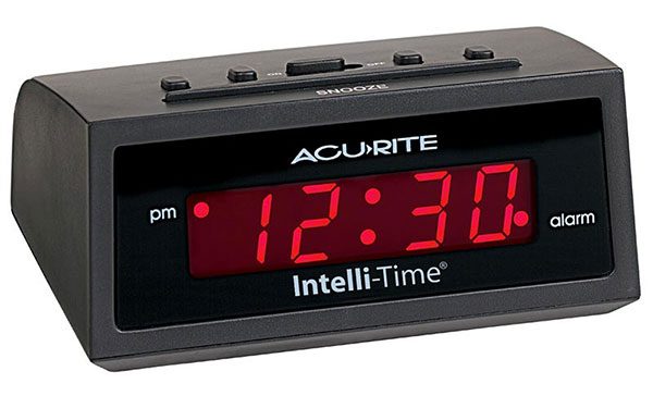
A great example of such a display is your classic digital alarm clock:
![Figure 1: A classic digital alarm clock that contains four seven-segment displays to represent the time of day.]()
Figure 1: A classic digital alarm clock that contains four seven-segment displays to represent the time of day.
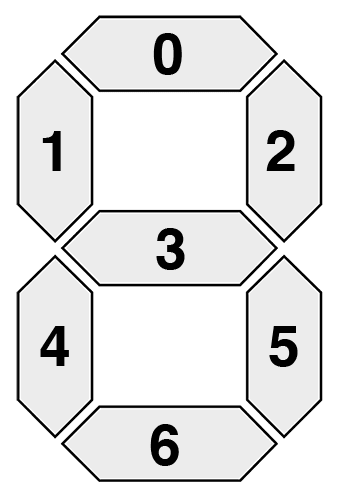
Each digit on the alarm clock is represented by a seven-segment component just like the one below:
![Figure 2: An example of a single seven-segment display. Each segment can be turned "on" or "off" to represent a particular digit.]()
Figure 2: An example of a single seven-segment display. Each segment can be turned “on” or “off” to represent a particular digit (source: Wikipedia).
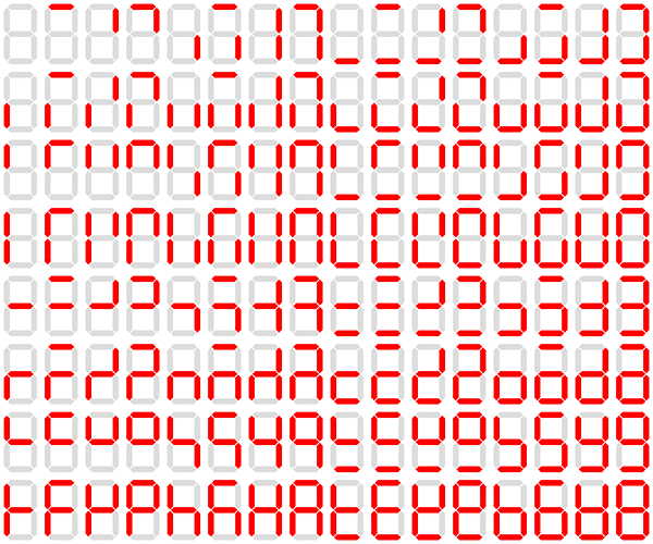
Sevent-segment displays can take on a total of 128 possible states:
![Figure 3: A seven-segment display is capable of 128 possible states (source: Wikipedia).]()
Figure 3: A seven-segment display is capable of 128 possible states (source: Wikipedia).
Luckily for us, we are only interested in ten of them — the digits zero to nine:
![Figure 4: However, for the task of digit recognition we only need to recognize ten of these states.]()
Figure 4: For the task of digit recognition we only need to recognize ten of these states.
Our goal is to write OpenCV and Python code to recognize each of these ten digit states in an image.
Planning the OpenCV digit recognizer
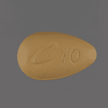
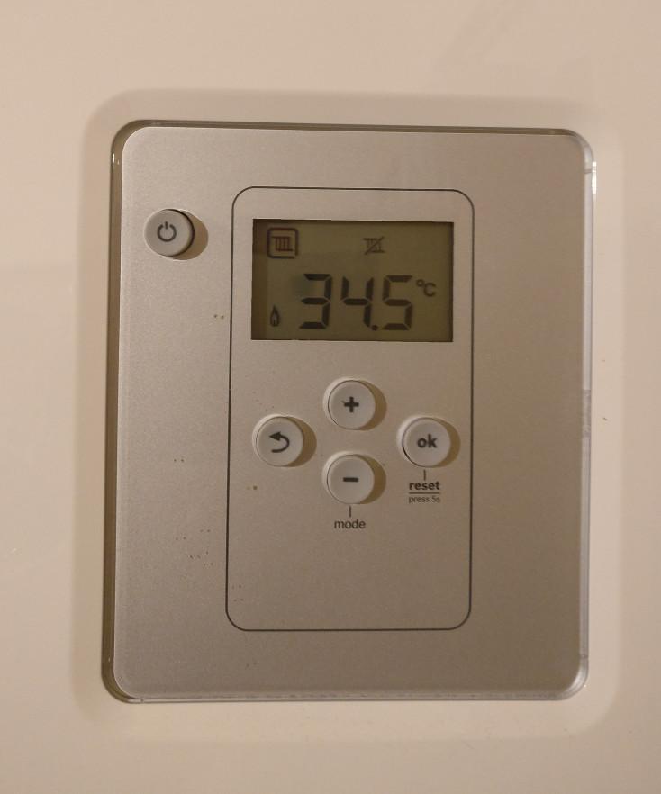
Just like in the original post on /r/computervision, we’ll be using the thermostat image as input:
![Figure 5: Our example input image. Our goal is to recognize the digits on the thermostat using OpenCV and Python.]()
Figure 5: Our example input image. Our goal is to recognize the digits on the thermostat using OpenCV and Python.
Whenever I am trying to recognize/identify object(s) in an image I first take a few minutes to assess the problem. Given that my end goal is to recognize the digits on the LCD display I know I need to:
- Step #1: Localize the LCD on the thermostat. This can be done using edge detection since there is enough contrast between the plastic shell and the LCD.
- Step #2: Extract the LCD. Given an input edge map I can find contours and look for outlines with a rectangular shape — the largest rectangular region should correspond to the LCD. A perspective transform will give me a nice extraction of the LCD.
- Step #3: Extract the digit regions. Once I have the LCD itself I can focus on extracting the digits. Since there seems to be contrast between the digit regions and the background of the LCD I’m confident that thresholding and morphological operations can accomplish this.
- Step #4: Identify the digits. Recognizing the actual digits with OpenCV will involve dividing the digit ROI into seven segments. From there I can apply pixel counting on the thresholded image to determine if a given segment is “on” or “off”.
So see how we can accomplish this four-step process to digit recognition with OpenCV and Python, keep reading.
Recognizing digits with computer vision and OpenCV
Let’s go ahead and get this example started.
Open up a new file, name it
recognize_digits.py
, and insert the following code:
# import the necessary packages
from imutils.perspective import four_point_transform
from imutils import contours
import imutils
import cv2

# define the dictionary of digit segments so we can identify
# each digit on the thermostat
DIGITS_LOOKUP = {
	(1, 1, 1, 0, 1, 1, 1): 0,
	(0, 0, 1, 0, 0, 1, 0): 1,
	(1, 0, 1, 1, 1, 1, 0): 2,
	(1, 0, 1, 1, 0, 1, 1): 3,
	(0, 1, 1, 1, 0, 1, 0): 4,
	(1, 1, 0, 1, 0, 1, 1): 5,
	(1, 1, 0, 1, 1, 1, 1): 6,
	(1, 0, 1, 0, 0, 1, 0): 7,
	(1, 1, 1, 1, 1, 1, 1): 8,
	(1, 1, 1, 1, 0, 1, 1): 9
}
Lines 2-5 import our required Python packages. We’ll be using imutils, my series of convenience functions to make working with OpenCV + Python easier. If you don’t already have
imutils
installed, you should take a second now to install the package on your system using
pip
:
$ pip install imutils
Lines 9-20 define a Python dictionary named
DIGITS_LOOKUP
. Inspired by the approach of /u/Jonno_FTW in the Reddit thread, we can easily define this lookup table where:
- They key to the table is the seven-segment array. A one in the array indicates that the given segment is on and a zero indicates that the segment is off.
- The value is the actual numerical digit itself: 0-9.
Once we identify the segments in the thermostat display we can pass the array into our
DIGITS_LOOKUP
table and obtain the digit value.
For reference, this dictionary uses the same segment ordering as in Figure 2 above.
Let’s continue with our example:
# import the necessary packages
from imutils.perspective import four_point_transform
from imutils import contours
import imutils
import cv2

# define the dictionary of digit segments so we can identify
# each digit on the thermostat
DIGITS_LOOKUP = {
	(1, 1, 1, 0, 1, 1, 1): 0,
	(0, 0, 1, 0, 0, 1, 0): 1,
	(1, 0, 1, 1, 1, 1, 0): 2,
	(1, 0, 1, 1, 0, 1, 1): 3,
	(0, 1, 1, 1, 0, 1, 0): 4,
	(1, 1, 0, 1, 0, 1, 1): 5,
	(1, 1, 0, 1, 1, 1, 1): 6,
	(1, 0, 1, 0, 0, 1, 0): 7,
	(1, 1, 1, 1, 1, 1, 1): 8,
	(1, 1, 1, 1, 0, 1, 1): 9
}

# load the example image
image = cv2.imread("example.jpg")

# pre-process the image by resizing it, converting it to
# graycale, blurring it, and computing an edge map
image = imutils.resize(image, height=500)
gray = cv2.cvtColor(image, cv2.COLOR_BGR2GRAY)
blurred = cv2.GaussianBlur(gray, (5, 5), 0)
edged = cv2.Canny(blurred, 50, 200, 255)
Line 23 loads our image from disk.
We then pre-process the image on Lines 27-30 by:
- Resizing it.
- Converting the image to grayscale.
- Applying Gaussian blurring with a 5×5 kernel to reduce high-frequency noise.
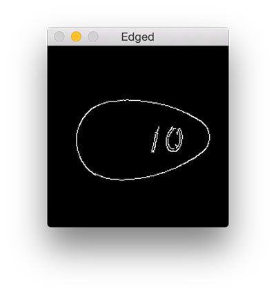
- Computing the edge map via the Canny edge detector.
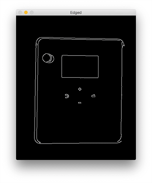
After applying these pre-processing steps our edge map looks like this:
![Figure 6: Applying image processing steps to compute the edge map of our input image.]()
Figure 6: Applying image processing steps to compute the edge map of our input image.
Notice how the outlines of the LCD are clearly visible — this accomplishes Step #1.
We can now move on to Step #2, extracting the LCD itself:
# import the necessary packages
from imutils.perspective import four_point_transform
from imutils import contours
import imutils
import cv2

# define the dictionary of digit segments so we can identify
# each digit on the thermostat
DIGITS_LOOKUP = {
	(1, 1, 1, 0, 1, 1, 1): 0,
	(0, 0, 1, 0, 0, 1, 0): 1,
	(1, 0, 1, 1, 1, 1, 0): 2,
	(1, 0, 1, 1, 0, 1, 1): 3,
	(0, 1, 1, 1, 0, 1, 0): 4,
	(1, 1, 0, 1, 0, 1, 1): 5,
	(1, 1, 0, 1, 1, 1, 1): 6,
	(1, 0, 1, 0, 0, 1, 0): 7,
	(1, 1, 1, 1, 1, 1, 1): 8,
	(1, 1, 1, 1, 0, 1, 1): 9
}

# load the example image
image = cv2.imread("example.jpg")

# pre-process the image by resizing it, converting it to
# graycale, blurring it, and computing an edge map
image = imutils.resize(image, height=500)
gray = cv2.cvtColor(image, cv2.COLOR_BGR2GRAY)
blurred = cv2.GaussianBlur(gray, (5, 5), 0)
edged = cv2.Canny(blurred, 50, 200, 255)

# find contours in the edge map, then sort them by their
# size in descending order
cnts = cv2.findContours(edged.copy(), cv2.RETR_EXTERNAL,
	cv2.CHAIN_APPROX_SIMPLE)
cnts = cnts[0] if imutils.is_cv2() else cnts[1]
cnts = sorted(cnts, key=cv2.contourArea, reverse=True)
displayCnt = None

# loop over the contours
for c in cnts:
	# approximate the contour
	peri = cv2.arcLength(c, True)
	approx = cv2.approxPolyDP(c, 0.02 * peri, True)

	# if the contour has four vertices, then we have found
	# the thermostat display
	if len(approx) == 4:
		displayCnt = approx
		break
In order to find the LCD regions, we need to extract the contours (i.e., outlines) of the regions in the edge map (Lines 35 and 35).
We then sort the contours by their area, ensuring that contours with a larger area are placed at the front of the list (Line 37).
Given our sorted contours list, we loop over them individually on Line 41 and apply contour approximation.
If our approximated contour has four vertices then we assume we have found the thermostat display (Lines 48-50). This is a reasonable assumption since the largest rectangular region in our input image should be the LCD itself.
After obtaining the four vertices we can extract the LCD via a four point perspective transform:
# import the necessary packages
from imutils.perspective import four_point_transform
from imutils import contours
import imutils
import cv2
# define the dictionary of digit segments so we can identify
# each digit on the thermostat
DIGITS_LOOKUP = {
(1, 1, 1, 0, 1, 1, 1): 0,
(0, 0, 1, 0, 0, 1, 0): 1,
(1, 0, 1, 1, 1, 1, 0): 2,
(1, 0, 1, 1, 0, 1, 1): 3,
(0, 1, 1, 1, 0, 1, 0): 4,
(1, 1, 0, 1, 0, 1, 1): 5,
(1, 1, 0, 1, 1, 1, 1): 6,
(1, 0, 1, 0, 0, 1, 0): 7,
(1, 1, 1, 1, 1, 1, 1): 8,
(1, 1, 1, 1, 0, 1, 1): 9
}
# load the example image
image = cv2.imread("example.jpg")
# pre-process the image by resizing it, converting it to
# graycale, blurring it, and computing an edge map
image = imutils.resize(image, height=500)
gray = cv2.cvtColor(image, cv2.COLOR_BGR2GRAY)
blurred = cv2.GaussianBlur(gray, (5, 5), 0)
edged = cv2.Canny(blurred, 50, 200, 255)
# find contours in the edge map, then sort them by their
# size in descending order
cnts = cv2.findContours(edged.copy(), cv2.RETR_EXTERNAL,
cv2.CHAIN_APPROX_SIMPLE)
cnts = cnts[0] if imutils.is_cv2() else cnts[1]
cnts = sorted(cnts, key=cv2.contourArea, reverse=True)
displayCnt = None
# loop over the contours
for c in cnts:
# approximate the contour
peri = cv2.arcLength(c, True)
approx = cv2.approxPolyDP(c, 0.02 * peri, True)
# if the contour has four vertices, then we have found
# the thermostat display
if len(approx) == 4:
displayCnt = approx
break
# extract the thermostat display, apply a perspective transform
# to it
warped = four_point_transform(gray, displayCnt.reshape(4, 2))
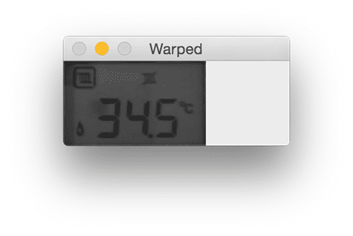
output = four_point_transform(image, displayCnt.reshape(4, 2))Applying this perspective transform gives us a top-down, birds-eye-view of the LCD:
![Figure 7: Applying a perspective transform to our image to obtain the LCD region.]()
Figure 7: Applying a perspective transform to our image to obtain the LCD region.
Obtaining this view of the LCD satisfies Step #2 — we are now ready to extract the digits from the LCD:
# import the necessary packages
from imutils.perspective import four_point_transform
from imutils import contours
import imutils
import cv2
# define the dictionary of digit segments so we can identify
# each digit on the thermostat
DIGITS_LOOKUP = {
(1, 1, 1, 0, 1, 1, 1): 0,
(0, 0, 1, 0, 0, 1, 0): 1,
(1, 0, 1, 1, 1, 1, 0): 2,
(1, 0, 1, 1, 0, 1, 1): 3,
(0, 1, 1, 1, 0, 1, 0): 4,
(1, 1, 0, 1, 0, 1, 1): 5,
(1, 1, 0, 1, 1, 1, 1): 6,
(1, 0, 1, 0, 0, 1, 0): 7,
(1, 1, 1, 1, 1, 1, 1): 8,
(1, 1, 1, 1, 0, 1, 1): 9
}
# load the example image
image = cv2.imread("example.jpg")
# pre-process the image by resizing it, converting it to
# graycale, blurring it, and computing an edge map
image = imutils.resize(image, height=500)
gray = cv2.cvtColor(image, cv2.COLOR_BGR2GRAY)
blurred = cv2.GaussianBlur(gray, (5, 5), 0)
edged = cv2.Canny(blurred, 50, 200, 255)
# find contours in the edge map, then sort them by their
# size in descending order
cnts = cv2.findContours(edged.copy(), cv2.RETR_EXTERNAL,
cv2.CHAIN_APPROX_SIMPLE)
cnts = cnts[0] if imutils.is_cv2() else cnts[1]
cnts = sorted(cnts, key=cv2.contourArea, reverse=True)
displayCnt = None
# loop over the contours
for c in cnts:
# approximate the contour
peri = cv2.arcLength(c, True)
approx = cv2.approxPolyDP(c, 0.02 * peri, True)
# if the contour has four vertices, then we have found
# the thermostat display
if len(approx) == 4:
displayCnt = approx
break
# extract the thermostat display, apply a perspective transform
# to it
warped = four_point_transform(gray, displayCnt.reshape(4, 2))
output = four_point_transform(image, displayCnt.reshape(4, 2))
# threshold the warped image, then apply a series of morphological
# operations to cleanup the thresholded image
thresh = cv2.threshold(warped, 0, 255,
cv2.THRESH_BINARY_INV | cv2.THRESH_OTSU)[1]
kernel = cv2.getStructuringElement(cv2.MORPH_ELLIPSE, (1, 5))
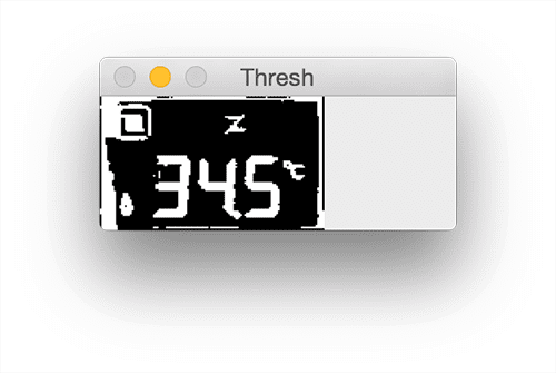
thresh = cv2.morphologyEx(thresh, cv2.MORPH_OPEN, kernel)To obtain the digits themselves we need to threshold the
warped
image (
Lines 59 and 60) to reveal the dark regions (i.e., digits) against the lighter background (i.e., the background of the LCD display):
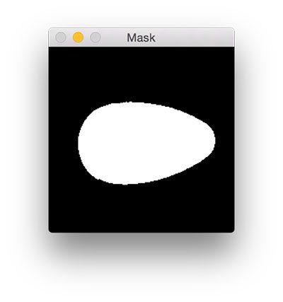
![Figure 8: Thresholding LCD allows us to segment the dark regions (digits/symbols) from the lighter background (the LCD display itself).]()
Figure 8: Thresholding LCD allows us to segment the dark regions (digits/symbols) from the lighter background (the LCD display itself).
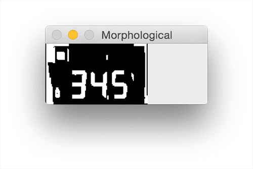
We then apply a series of morphological operations to clean up the thresholded image (Lines 61 and 62):
![Figure 9: Applying a series of morphological operations cleans up our thresholded LCD and will allow us to segment out each of the digits.]()
Figure 9: Applying a series of morphological operations cleans up our thresholded LCD and will allow us to segment out each of the digits.
Now that we have a nice segmented image we once again need to apply contour filtering, only this time we are looking for the actual digits:
# import the necessary packages
from imutils.perspective import four_point_transform
from imutils import contours
import imutils
import cv2

# define the dictionary of digit segments so we can identify
# each digit on the thermostat
DIGITS_LOOKUP = {
	(1, 1, 1, 0, 1, 1, 1): 0,
	(0, 0, 1, 0, 0, 1, 0): 1,
	(1, 0, 1, 1, 1, 1, 0): 2,
	(1, 0, 1, 1, 0, 1, 1): 3,
	(0, 1, 1, 1, 0, 1, 0): 4,
	(1, 1, 0, 1, 0, 1, 1): 5,
	(1, 1, 0, 1, 1, 1, 1): 6,
	(1, 0, 1, 0, 0, 1, 0): 7,
	(1, 1, 1, 1, 1, 1, 1): 8,
	(1, 1, 1, 1, 0, 1, 1): 9
}

# load the example image
image = cv2.imread("example.jpg")

# pre-process the image by resizing it, converting it to
# graycale, blurring it, and computing an edge map
image = imutils.resize(image, height=500)
gray = cv2.cvtColor(image, cv2.COLOR_BGR2GRAY)
blurred = cv2.GaussianBlur(gray, (5, 5), 0)
edged = cv2.Canny(blurred, 50, 200, 255)

# find contours in the edge map, then sort them by their
# size in descending order
cnts = cv2.findContours(edged.copy(), cv2.RETR_EXTERNAL,
	cv2.CHAIN_APPROX_SIMPLE)
cnts = cnts[0] if imutils.is_cv2() else cnts[1]
cnts = sorted(cnts, key=cv2.contourArea, reverse=True)
displayCnt = None

# loop over the contours
for c in cnts:
	# approximate the contour
	peri = cv2.arcLength(c, True)
	approx = cv2.approxPolyDP(c, 0.02 * peri, True)

	# if the contour has four vertices, then we have found
	# the thermostat display
	if len(approx) == 4:
		displayCnt = approx
		break

# extract the thermostat display, apply a perspective transform
# to it
warped = four_point_transform(gray, displayCnt.reshape(4, 2))
output = four_point_transform(image, displayCnt.reshape(4, 2))

# threshold the warped image, then apply a series of morphological
# operations to cleanup the thresholded image
thresh = cv2.threshold(warped, 0, 255,
	cv2.THRESH_BINARY_INV | cv2.THRESH_OTSU)[1]
kernel = cv2.getStructuringElement(cv2.MORPH_ELLIPSE, (1, 5))
thresh = cv2.morphologyEx(thresh, cv2.MORPH_OPEN, kernel)

# find contours in the thresholded image, then initialize the
# digit contours lists
cnts = cv2.findContours(thresh.copy(), cv2.RETR_EXTERNAL,
	cv2.CHAIN_APPROX_SIMPLE)
cnts = cnts[0] if imutils.is_cv2() else cnts[1]
digitCnts = []

# loop over the digit area candidates
for c in cnts:
	# compute the bounding box of the contour
	(x, y, w, h) = cv2.boundingRect(c)

	# if the contour is sufficiently large, it must be a digit
	if w >= 15 and (h >= 30 and h <= 40):
		digitCnts.append(c)
To accomplish this we find contours in our thresholded image (Lines 66 and 67). We also initialize the
digitsCnts
list on
Line 69 — this list will store the contours of the digits themselves.
Line 72 starts looping over each of the contours.
For each contour, we compute the bounding box (Line 74), ensure the width and height are of an acceptable size, and if so, update the
digitsCnts
list (
Lines 77 and 78).
Note: Determining the appropriate width and height constraints requires a few rounds of trial and error. I would suggest looping over each of the contours, drawing them individually, and inspecting their dimensions. Doing this process ensures you can find commonalities across digit contour properties.
If we were to loop over the contours inside
digitsCnts
and draw the bounding box on our image, the result would look like this:
![Figure 10: Drawing the bounding box of each of the digits on the LCD.]()
Figure 10: Drawing the bounding box of each of the digits on the LCD.
Sure enough, we have found the digits on the LCD!
The final step is to actually identify each of the digits:
# import the necessary packages
from imutils.perspective import four_point_transform
from imutils import contours
import imutils
import cv2

# define the dictionary of digit segments so we can identify
# each digit on the thermostat
DIGITS_LOOKUP = {
	(1, 1, 1, 0, 1, 1, 1): 0,
	(0, 0, 1, 0, 0, 1, 0): 1,
	(1, 0, 1, 1, 1, 1, 0): 2,
	(1, 0, 1, 1, 0, 1, 1): 3,
	(0, 1, 1, 1, 0, 1, 0): 4,
	(1, 1, 0, 1, 0, 1, 1): 5,
	(1, 1, 0, 1, 1, 1, 1): 6,
	(1, 0, 1, 0, 0, 1, 0): 7,
	(1, 1, 1, 1, 1, 1, 1): 8,
	(1, 1, 1, 1, 0, 1, 1): 9
}

# load the example image
image = cv2.imread("example.jpg")

# pre-process the image by resizing it, converting it to
# graycale, blurring it, and computing an edge map
image = imutils.resize(image, height=500)
gray = cv2.cvtColor(image, cv2.COLOR_BGR2GRAY)
blurred = cv2.GaussianBlur(gray, (5, 5), 0)
edged = cv2.Canny(blurred, 50, 200, 255)

# find contours in the edge map, then sort them by their
# size in descending order
cnts = cv2.findContours(edged.copy(), cv2.RETR_EXTERNAL,
	cv2.CHAIN_APPROX_SIMPLE)
cnts = cnts[0] if imutils.is_cv2() else cnts[1]
cnts = sorted(cnts, key=cv2.contourArea, reverse=True)
displayCnt = None

# loop over the contours
for c in cnts:
	# approximate the contour
	peri = cv2.arcLength(c, True)
	approx = cv2.approxPolyDP(c, 0.02 * peri, True)

	# if the contour has four vertices, then we have found
	# the thermostat display
	if len(approx) == 4:
		displayCnt = approx
		break

# extract the thermostat display, apply a perspective transform
# to it
warped = four_point_transform(gray, displayCnt.reshape(4, 2))
output = four_point_transform(image, displayCnt.reshape(4, 2))

# threshold the warped image, then apply a series of morphological
# operations to cleanup the thresholded image
thresh = cv2.threshold(warped, 0, 255,
	cv2.THRESH_BINARY_INV | cv2.THRESH_OTSU)[1]
kernel = cv2.getStructuringElement(cv2.MORPH_ELLIPSE, (1, 5))
thresh = cv2.morphologyEx(thresh, cv2.MORPH_OPEN, kernel)

# find contours in the thresholded image, then initialize the
# digit contours lists
cnts = cv2.findContours(thresh.copy(), cv2.RETR_EXTERNAL,
	cv2.CHAIN_APPROX_SIMPLE)
cnts = cnts[0] if imutils.is_cv2() else cnts[1]
digitCnts = []

# loop over the digit area candidates
for c in cnts:
	# compute the bounding box of the contour
	(x, y, w, h) = cv2.boundingRect(c)

	# if the contour is sufficiently large, it must be a digit
	if w >= 15 and (h >= 30 and h <= 40):
		digitCnts.append(c)

# sort the contours from left-to-right, then initialize the
# actual digits themselves
digitCnts = contours.sort_contours(digitCnts,
	method="left-to-right")[0]
digits = []
Here we are simply sorting our digit contours from left-to-right based on their (x, y)-coordinates.
This sorting step is necessary as there are no guarantees that the contours are already sorted from left-to-right (the same direction in which we would read the digits).
Next, comes the actual digit recognition process:
# import the necessary packages
from imutils.perspective import four_point_transform
from imutils import contours
import imutils
import cv2

# define the dictionary of digit segments so we can identify
# each digit on the thermostat
DIGITS_LOOKUP = {
	(1, 1, 1, 0, 1, 1, 1): 0,
	(0, 0, 1, 0, 0, 1, 0): 1,
	(1, 0, 1, 1, 1, 1, 0): 2,
	(1, 0, 1, 1, 0, 1, 1): 3,
	(0, 1, 1, 1, 0, 1, 0): 4,
	(1, 1, 0, 1, 0, 1, 1): 5,
	(1, 1, 0, 1, 1, 1, 1): 6,
	(1, 0, 1, 0, 0, 1, 0): 7,
	(1, 1, 1, 1, 1, 1, 1): 8,
	(1, 1, 1, 1, 0, 1, 1): 9
}

# load the example image
image = cv2.imread("example.jpg")

# pre-process the image by resizing it, converting it to
# graycale, blurring it, and computing an edge map
image = imutils.resize(image, height=500)
gray = cv2.cvtColor(image, cv2.COLOR_BGR2GRAY)
blurred = cv2.GaussianBlur(gray, (5, 5), 0)
edged = cv2.Canny(blurred, 50, 200, 255)

# find contours in the edge map, then sort them by their
# size in descending order
cnts = cv2.findContours(edged.copy(), cv2.RETR_EXTERNAL,
	cv2.CHAIN_APPROX_SIMPLE)
cnts = cnts[0] if imutils.is_cv2() else cnts[1]
cnts = sorted(cnts, key=cv2.contourArea, reverse=True)
displayCnt = None

# loop over the contours
for c in cnts:
	# approximate the contour
	peri = cv2.arcLength(c, True)
	approx = cv2.approxPolyDP(c, 0.02 * peri, True)

	# if the contour has four vertices, then we have found
	# the thermostat display
	if len(approx) == 4:
		displayCnt = approx
		break

# extract the thermostat display, apply a perspective transform
# to it
warped = four_point_transform(gray, displayCnt.reshape(4, 2))
output = four_point_transform(image, displayCnt.reshape(4, 2))

# threshold the warped image, then apply a series of morphological
# operations to cleanup the thresholded image
thresh = cv2.threshold(warped, 0, 255,
	cv2.THRESH_BINARY_INV | cv2.THRESH_OTSU)[1]
kernel = cv2.getStructuringElement(cv2.MORPH_ELLIPSE, (1, 5))
thresh = cv2.morphologyEx(thresh, cv2.MORPH_OPEN, kernel)

# find contours in the thresholded image, then initialize the
# digit contours lists
cnts = cv2.findContours(thresh.copy(), cv2.RETR_EXTERNAL,
	cv2.CHAIN_APPROX_SIMPLE)
cnts = cnts[0] if imutils.is_cv2() else cnts[1]
digitCnts = []

# loop over the digit area candidates
for c in cnts:
	# compute the bounding box of the contour
	(x, y, w, h) = cv2.boundingRect(c)

	# if the contour is sufficiently large, it must be a digit
	if w >= 15 and (h >= 30 and h <= 40):
		digitCnts.append(c)

# sort the contours from left-to-right, then initialize the
# actual digits themselves
digitCnts = contours.sort_contours(digitCnts,
	method="left-to-right")[0]
digits = []

# loop over each of the digits
for c in digitCnts:
	# extract the digit ROI
	(x, y, w, h) = cv2.boundingRect(c)
	roi = thresh[y:y + h, x:x + w]

	# compute the width and height of each of the 7 segments
	# we are going to examine
	(roiH, roiW) = roi.shape
	(dW, dH) = (int(roiW * 0.25), int(roiH * 0.15))
	dHC = int(roiH * 0.05)

	# define the set of 7 segments
	segments = [
		((0, 0), (w, dH)),	# top
		((0, 0), (dW, h // 2)),	# top-left
		((w - dW, 0), (w, h // 2)),	# top-right
		((0, (h // 2) - dHC) , (w, (h // 2) + dHC)), # center
		((0, h // 2), (dW, h)),	# bottom-left
		((w - dW, h // 2), (w, h)),	# bottom-right
		((0, h - dH), (w, h))	# bottom
	]
	on = [0] * len(segments)
We start looping over each of the digit contours on Line 87.
For each of these regions, we compute the bounding box and extract the digit ROI (Lines 89 and 90).
I have included a GIF animation of each of these digit ROIs below:
![Figure 11: Extracting each individual digit ROI by computing the bounding box and applying NumPy array slicing.]()
Figure 11: Extracting each individual digit ROI by computing the bounding box and applying NumPy array slicing.
Given the digit ROI we now need to localize and extract the seven segments of the digit display.
Lines 94-96 compute the approximate width and height of each segment based on the ROI dimensions.
We then define a list of (x, y)-coordinates that correspond to the seven segments on Lines 99-107. This list follows the same order of segments as Figure 2 above.
Here is an example GIF animation that draws a green box over the current segment being investigated:
![Figure 12: An example of drawing the segment ROI for each of the seven segments of the digit.]()
Figure 12: An example of drawing the segment ROI for each of the seven segments of the digit.
Finally, Line 108 initializes our
on
list — a value of
one inside this list indicates that a given segment is turned “on” while a value of
zero indicates the segment is “off”.
Given the (x, y)-coordinates of the seven display segments, identifying a whether a segment is on or off is fairly easy:
# import the necessary packages
from imutils.perspective import four_point_transform
from imutils import contours
import imutils
import cv2

# define the dictionary of digit segments so we can identify
# each digit on the thermostat
DIGITS_LOOKUP = {
	(1, 1, 1, 0, 1, 1, 1): 0,
	(0, 0, 1, 0, 0, 1, 0): 1,
	(1, 0, 1, 1, 1, 1, 0): 2,
	(1, 0, 1, 1, 0, 1, 1): 3,
	(0, 1, 1, 1, 0, 1, 0): 4,
	(1, 1, 0, 1, 0, 1, 1): 5,
	(1, 1, 0, 1, 1, 1, 1): 6,
	(1, 0, 1, 0, 0, 1, 0): 7,
	(1, 1, 1, 1, 1, 1, 1): 8,
	(1, 1, 1, 1, 0, 1, 1): 9
}

# load the example image
image = cv2.imread("example.jpg")

# pre-process the image by resizing it, converting it to
# graycale, blurring it, and computing an edge map
image = imutils.resize(image, height=500)
gray = cv2.cvtColor(image, cv2.COLOR_BGR2GRAY)
blurred = cv2.GaussianBlur(gray, (5, 5), 0)
edged = cv2.Canny(blurred, 50, 200, 255)

# find contours in the edge map, then sort them by their
# size in descending order
cnts = cv2.findContours(edged.copy(), cv2.RETR_EXTERNAL,
	cv2.CHAIN_APPROX_SIMPLE)
cnts = cnts[0] if imutils.is_cv2() else cnts[1]
cnts = sorted(cnts, key=cv2.contourArea, reverse=True)
displayCnt = None

# loop over the contours
for c in cnts:
	# approximate the contour
	peri = cv2.arcLength(c, True)
	approx = cv2.approxPolyDP(c, 0.02 * peri, True)

	# if the contour has four vertices, then we have found
	# the thermostat display
	if len(approx) == 4:
		displayCnt = approx
		break

# extract the thermostat display, apply a perspective transform
# to it
warped = four_point_transform(gray, displayCnt.reshape(4, 2))
output = four_point_transform(image, displayCnt.reshape(4, 2))

# threshold the warped image, then apply a series of morphological
# operations to cleanup the thresholded image
thresh = cv2.threshold(warped, 0, 255,
	cv2.THRESH_BINARY_INV | cv2.THRESH_OTSU)[1]
kernel = cv2.getStructuringElement(cv2.MORPH_ELLIPSE, (1, 5))
thresh = cv2.morphologyEx(thresh, cv2.MORPH_OPEN, kernel)

# find contours in the thresholded image, then initialize the
# digit contours lists
cnts = cv2.findContours(thresh.copy(), cv2.RETR_EXTERNAL,
	cv2.CHAIN_APPROX_SIMPLE)
cnts = cnts[0] if imutils.is_cv2() else cnts[1]
digitCnts = []

# loop over the digit area candidates
for c in cnts:
	# compute the bounding box of the contour
	(x, y, w, h) = cv2.boundingRect(c)

	# if the contour is sufficiently large, it must be a digit
	if w >= 15 and (h >= 30 and h <= 40):
		digitCnts.append(c)

# sort the contours from left-to-right, then initialize the
# actual digits themselves
digitCnts = contours.sort_contours(digitCnts,
	method="left-to-right")[0]
digits = []

# loop over each of the digits
for c in digitCnts:
	# extract the digit ROI
	(x, y, w, h) = cv2.boundingRect(c)
	roi = thresh[y:y + h, x:x + w]

	# compute the width and height of each of the 7 segments
	# we are going to examine
	(roiH, roiW) = roi.shape
	(dW, dH) = (int(roiW * 0.25), int(roiH * 0.15))
	dHC = int(roiH * 0.05)

	# define the set of 7 segments
	segments = [
		((0, 0), (w, dH)),	# top
		((0, 0), (dW, h // 2)),	# top-left
		((w - dW, 0), (w, h // 2)),	# top-right
		((0, (h // 2) - dHC) , (w, (h // 2) + dHC)), # center
		((0, h // 2), (dW, h)),	# bottom-left
		((w - dW, h // 2), (w, h)),	# bottom-right
		((0, h - dH), (w, h))	# bottom
	]
	on = [0] * len(segments)

	# loop over the segments
	for (i, ((xA, yA), (xB, yB))) in enumerate(segments):
		# extract the segment ROI, count the total number of
		# thresholded pixels in the segment, and then compute
		# the area of the segment
		segROI = roi[yA:yB, xA:xB]
		total = cv2.countNonZero(segROI)
		area = (xB - xA) * (yB - yA)

		# if the total number of non-zero pixels is greater than
		# 50% of the area, mark the segment as "on"
		if total / float(area) > 0.5:
			on[i]= 1

	# lookup the digit and draw it on the image
	digit = DIGITS_LOOKUP[tuple(on)]
	digits.append(digit)
	cv2.rectangle(output, (x, y), (x + w, y + h), (0, 255, 0), 1)
	cv2.putText(output, str(digit), (x - 10, y - 10),
		cv2.FONT_HERSHEY_SIMPLEX, 0.65, (0, 255, 0), 2)
We start looping over the (x, y)-coordinates of each segment on Line 111.
We extract the segment ROI on Line 115, followed by computing the number of non-zero pixels on Line 116 (i.e., the number of pixels in the segment that are “on”).
If the ratio of non-zero pixels to the total area of the segment is greater than 50% then we can assume the segment is “on” and update our
on
list accordingly (
Lines 121 and 122).
After looping over the seven segments we can pass the
on
list to
DIGITS_LOOKUP
to obtain the digit itself.
We then draw a bounding box around the digit and display the digit on the
output
image.
Finally, our last code block prints the digit to our screen and displays the output image:
# import the necessary packages
from imutils.perspective import four_point_transform
from imutils import contours
import imutils
import cv2
# define the dictionary of digit segments so we can identify
# each digit on the thermostat
DIGITS_LOOKUP = {
(1, 1, 1, 0, 1, 1, 1): 0,
(0, 0, 1, 0, 0, 1, 0): 1,
(1, 0, 1, 1, 1, 1, 0): 2,
(1, 0, 1, 1, 0, 1, 1): 3,
(0, 1, 1, 1, 0, 1, 0): 4,
(1, 1, 0, 1, 0, 1, 1): 5,
(1, 1, 0, 1, 1, 1, 1): 6,
(1, 0, 1, 0, 0, 1, 0): 7,
(1, 1, 1, 1, 1, 1, 1): 8,
(1, 1, 1, 1, 0, 1, 1): 9
}
# load the example image
image = cv2.imread("example.jpg")
# pre-process the image by resizing it, converting it to
# graycale, blurring it, and computing an edge map
image = imutils.resize(image, height=500)
gray = cv2.cvtColor(image, cv2.COLOR_BGR2GRAY)
blurred = cv2.GaussianBlur(gray, (5, 5), 0)
edged = cv2.Canny(blurred, 50, 200, 255)
# find contours in the edge map, then sort them by their
# size in descending order
cnts = cv2.findContours(edged.copy(), cv2.RETR_EXTERNAL,
cv2.CHAIN_APPROX_SIMPLE)
cnts = cnts[0] if imutils.is_cv2() else cnts[1]
cnts = sorted(cnts, key=cv2.contourArea, reverse=True)
displayCnt = None
# loop over the contours
for c in cnts:
# approximate the contour
peri = cv2.arcLength(c, True)
approx = cv2.approxPolyDP(c, 0.02 * peri, True)
# if the contour has four vertices, then we have found
# the thermostat display
if len(approx) == 4:
displayCnt = approx
break
# extract the thermostat display, apply a perspective transform
# to it
warped = four_point_transform(gray, displayCnt.reshape(4, 2))
output = four_point_transform(image, displayCnt.reshape(4, 2))
# threshold the warped image, then apply a series of morphological
# operations to cleanup the thresholded image
thresh = cv2.threshold(warped, 0, 255,
cv2.THRESH_BINARY_INV | cv2.THRESH_OTSU)[1]
kernel = cv2.getStructuringElement(cv2.MORPH_ELLIPSE, (1, 5))
thresh = cv2.morphologyEx(thresh, cv2.MORPH_OPEN, kernel)
# find contours in the thresholded image, then initialize the
# digit contours lists
cnts = cv2.findContours(thresh.copy(), cv2.RETR_EXTERNAL,
cv2.CHAIN_APPROX_SIMPLE)
cnts = cnts[0] if imutils.is_cv2() else cnts[1]
digitCnts = []
# loop over the digit area candidates
for c in cnts:
# compute the bounding box of the contour
(x, y, w, h) = cv2.boundingRect(c)
# if the contour is sufficiently large, it must be a digit
if w >= 15 and (h >= 30 and h <= 40):
digitCnts.append(c)
# sort the contours from left-to-right, then initialize the
# actual digits themselves
digitCnts = contours.sort_contours(digitCnts,
method="left-to-right")[0]
digits = []
# loop over each of the digits
for c in digitCnts:
# extract the digit ROI
(x, y, w, h) = cv2.boundingRect(c)
roi = thresh[y:y + h, x:x + w]
# compute the width and height of each of the 7 segments
# we are going to examine
(roiH, roiW) = roi.shape
(dW, dH) = (int(roiW * 0.25), int(roiH * 0.15))
dHC = int(roiH * 0.05)
# define the set of 7 segments
segments = [
((0, 0), (w, dH)), # top
((0, 0), (dW, h // 2)), # top-left
((w - dW, 0), (w, h // 2)), # top-right
((0, (h // 2) - dHC) , (w, (h // 2) + dHC)), # center
((0, h // 2), (dW, h)), # bottom-left
((w - dW, h // 2), (w, h)), # bottom-right
((0, h - dH), (w, h)) # bottom
]
on = [0] * len(segments)
# loop over the segments
for (i, ((xA, yA), (xB, yB))) in enumerate(segments):
# extract the segment ROI, count the total number of
# thresholded pixels in the segment, and then compute
# the area of the segment
segROI = roi[yA:yB, xA:xB]
total = cv2.countNonZero(segROI)
area = (xB - xA) * (yB - yA)
# if the total number of non-zero pixels is greater than
# 50% of the area, mark the segment as "on"
if total / float(area) > 0.5:
on[i]= 1
# lookup the digit and draw it on the image
digit = DIGITS_LOOKUP[tuple(on)]
digits.append(digit)
cv2.rectangle(output, (x, y), (x + w, y + h), (0, 255, 0), 1)
cv2.putText(output, str(digit), (x - 10, y - 10),
cv2.FONT_HERSHEY_SIMPLEX, 0.65, (0, 255, 0), 2)
# display the digits
print(u"{}{}.{} \u00b0C".format(*digits))
cv2.imshow("Input", image)
cv2.imshow("Output", output)
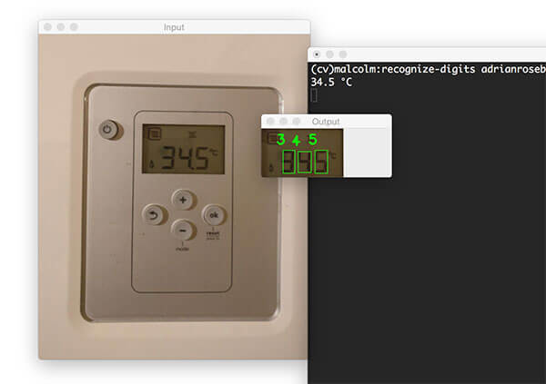
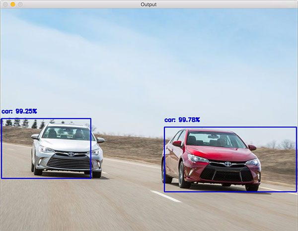
cv2.waitKey(0)Notice how we have been able to correctly recognize the digits on the LCD screen using Python and OpenCV:
![Figure 13: Correctly recognizing digits in images with OpenCV and Python.]()
Figure 13: Correctly recognizing digits in images with OpenCV and Python.
Summary
In today’s blog post I demonstrated how to utilize OpenCV and Python to recognize digits in images.
This approach is specifically intended for seven-segment displays (i.e., the digit displays you would typically see on a digital alarm clock).
By extracting each of the seven segments and applying basic thresholding and morphological operations we can determine which segments are “on” and which are “off”.
From there, we can look up the on/off segments in a Python dictionary data structure to quickly determine the actual digit — no machine learning required!
As I mentioned at the top of this blog post, applying computer vision to recognizing digits in a thermostat image tends to overcomplicate the problem itself — utilizing a data logging thermometer would be more reliable and require substantially less effort.
However, in the case that (1) you do not have access to a data logging sensor or (2) you simply want to hone and practice your computer vision/OpenCV skills, it’s often helpful to see a solution such as this one demonstrating how to solve the project.
I hope you enjoyed today’s post!
To be notified when future blog posts are published, be sure to enter your email address in the form below!
Downloads:
The post Recognizing digits with OpenCV and Python appeared first on PyImageSearch.


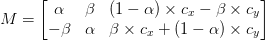
 degrees about some center
 ") coordinates at some scale (i.e., smaller or larger).
coordinates at some scale (i.e., smaller or larger). and
and  :
: and
and